
Historically, long-short equity factors have provided positive mean returns with low correlation to other assets. Most retail investors use long-only products, meaning they invest only in the long leg of the long-short factors. We will dissect factor returns into their long and short legs and further examine their performance in different states of the equity market—both bull markets and bear markets.
We will show that the value, profitability, investment, and momentum factors have provided much higher mean returns in bear markets compared to bull markets. The long leg of these factors has offered better diversification within a multifactor portfolio, while the short leg has driven superior performance in bear markets. The high bear market performance of these factors may be explained by a common factor, such as duration factors or the correction of mispricing that builds up during bull markets.
The size factor, associated with financial constraint factors and a lagged exposure to the market factor, has returns that are positively correlated with the market factor. The size factor has performed better during bull markets, while it has experienced negative mean returns in bear markets.
Cumulative factor returns in bull and bear markets
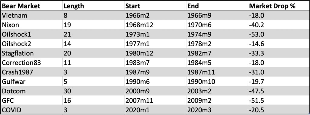
Geertsema & Lu classify U.S. bear markets in their paper Where is the risk in risk factors? Evidence from the Vietnam war to the COVID-19 pandemic [1], covering the period from July 1963 to March 2020. The table below (adapted from Table 1 of the Geertsema & Lu paper) shows the bear markets, which also apply to our data spanning from July 1963 to December 2021.
Our data spans 58.5 years, comprising 702 monthly returns, with 150 bear market months and 552 bull market months. In our data, the U.S. stock market spent about 79% of the time in bull markets and 21% in bear markets.
Our data is constructed using the market factor Market Minus Risk Free (Mkt-RF), the size factor Small Minus Big (SMB), and the value factor High Minus Low (HML) from the three-factor model, along with the profitability factor Robust Minus Weak (RMW) and the investment factor Conservative Minus Aggressive (CMA) from the five-factor model, and the momentum factor Up Minus Down (UMD) from the momentum factor data. All of our data is sourced from Kenneth French’s data library [2].
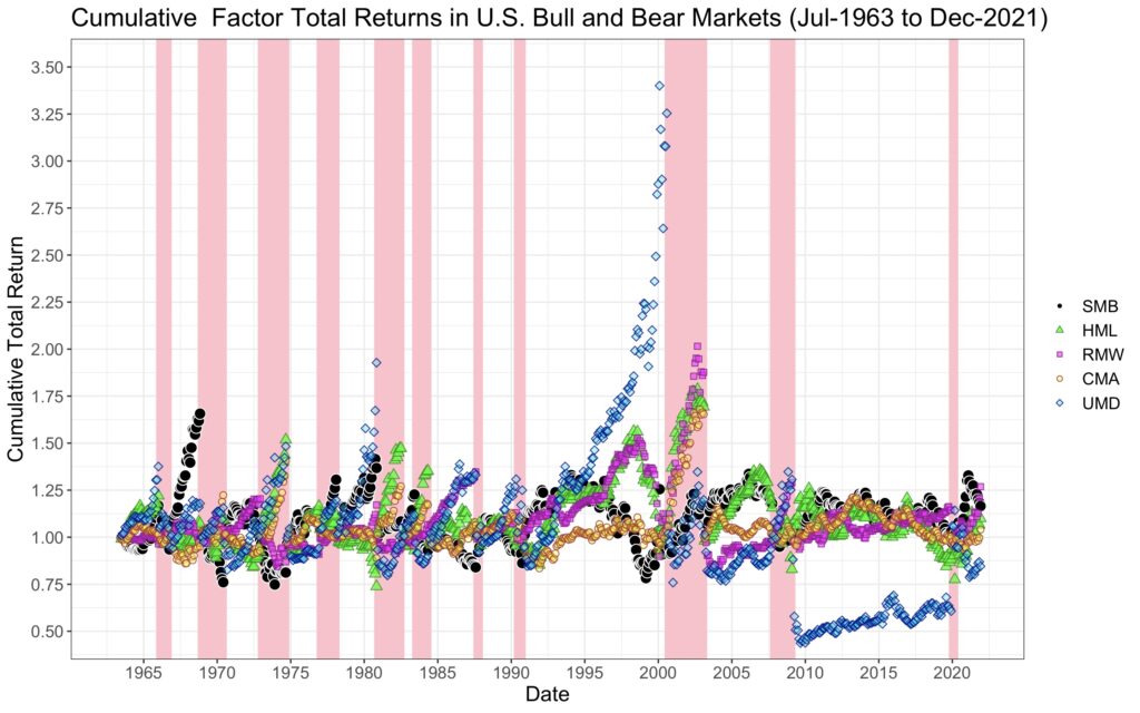
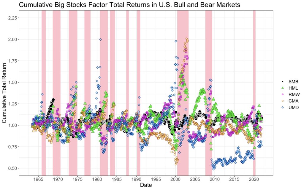
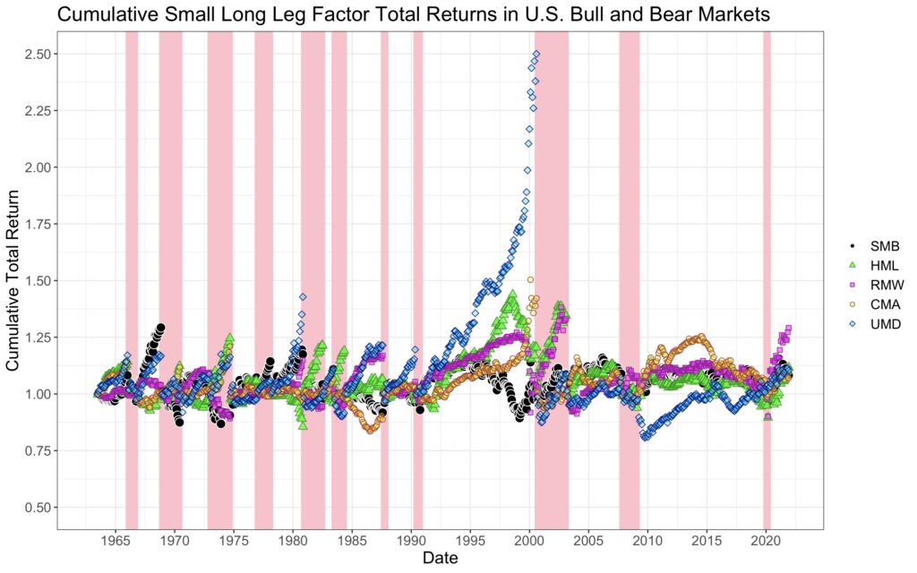
The figure below shows how a $1 investment in each factor (excluding the market factor), reset to $1 at the beginning of each bull and bear market, compounds over time. Bear markets are indicated with a pink background, while bull markets have a white background.
We can see that many factors have high returns when they are needed the most, i.e., in bear markets. The momentum factor provides some excellent runs but also experiences a big crash in the aftermath of the Global Financial Crisis (GFC).
Factors are constructed as long-short factors, meaning that the return is calculated as the difference between the long and short leg returns. For example, Fama and French construct factors by sorting both big and small stocks into three portfolios: value stocks are those with the highest book-to-market ratio (above the 70th percentile based on NYSE data), and growth stocks are those with the lowest book-to-market ratio (below the 30th percentile). The remaining stocks form a neutral portfolio. The value factor (HML) is then constructed as 1/2(Small Value + Big Value) – 1/2(Small Growth + Big Growth).
We can calculate the long and short leg returns separately by forming a neutral hedging portfolio between the long and short legs. This approach was used by Blitz, Baltussen, and van Vliet in their paper When Equity Factors Drop Their Shorts [3]. The authors utilize 2×3 bivariate portfolio sort data to construct their neutral hedging portfolio as 1/2 (simple average of the nine big stock portfolios of value, profitability, and investment factors) + 1/2 (simple average of the nine small stock portfolios of value, profitability, and investment factors).
Our neutral hedging portfolio is constructed similarly, except that it is based only on value factor data (utilizing the 2×3 bivariate portfolio sort data) and is defined as 1/2 ((1/3)*Big Value + (1/3)*Big Neutral + (1/3)*Big Growth) + 1/2 ((1/3)*Small Value + (1/3)*Small Neutral + (1/3)*Small Growth). In the case of tests involving only big stocks or small stocks, the neutral hedging portfolio consists exclusively of big or small stocks, respectively.
As an example, our long leg return for value factor is calculated as 1/2(Small Value + Big Value) – Neutral Hedging Portfolio, and the short leg return is calculated as Neutral Hedging Portfolio – 1/2(Small Growth + Big Growth). The neutral hedging portfolio return is always exactly halfway between big and small stock returns meaning that breakdown to long and short legs will not provide information about size factor returns. We therefore exclude size factor from most of the figures we present.
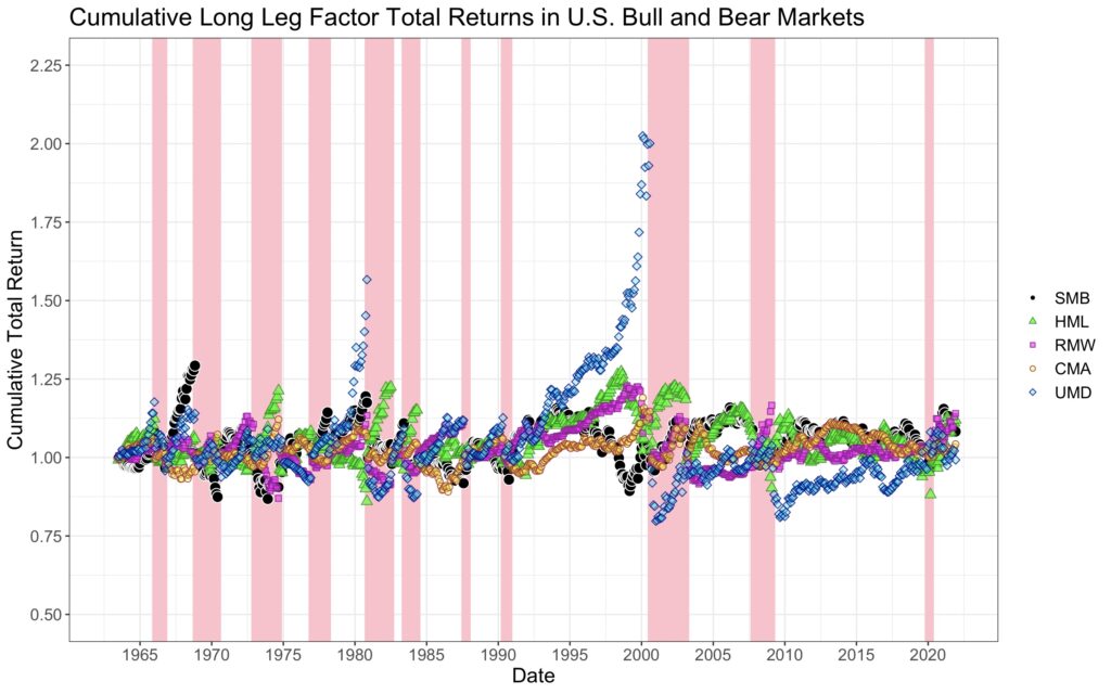
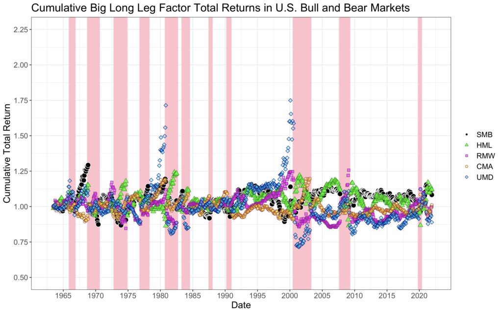
The next figure shows how a $1 investment compounds when we utilize the long leg of the factor returns. This simulates cumulative returns in excess of market returns (note, however, that this refers to our neutral hedging portfolio, not the typical value-weighted market portfolio) for long-only factor portfolios. Long-only investments are far more accessible and common for retail investors, who often invest through factor ETFs.
The striking difference from the previous long-short factor figure is that significant bear market returns are nearly absent here. On average, while the value factor still seems to deliver in bear markets, other factors do not perform as well. Momentum shows a notable crash during the tech bubble burst and in the aftermath of the GFC, but these crashes are not nearly as severe as observed with the long-short factors.
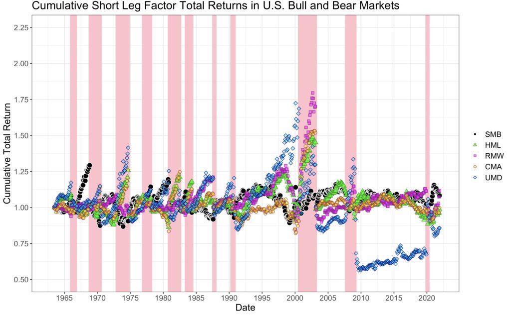
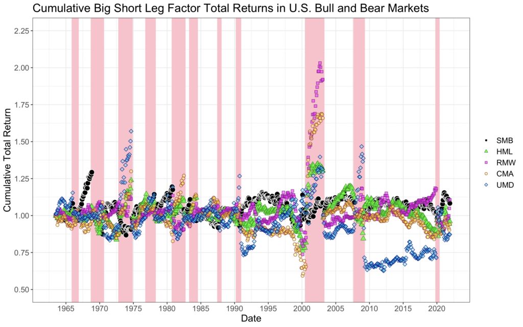
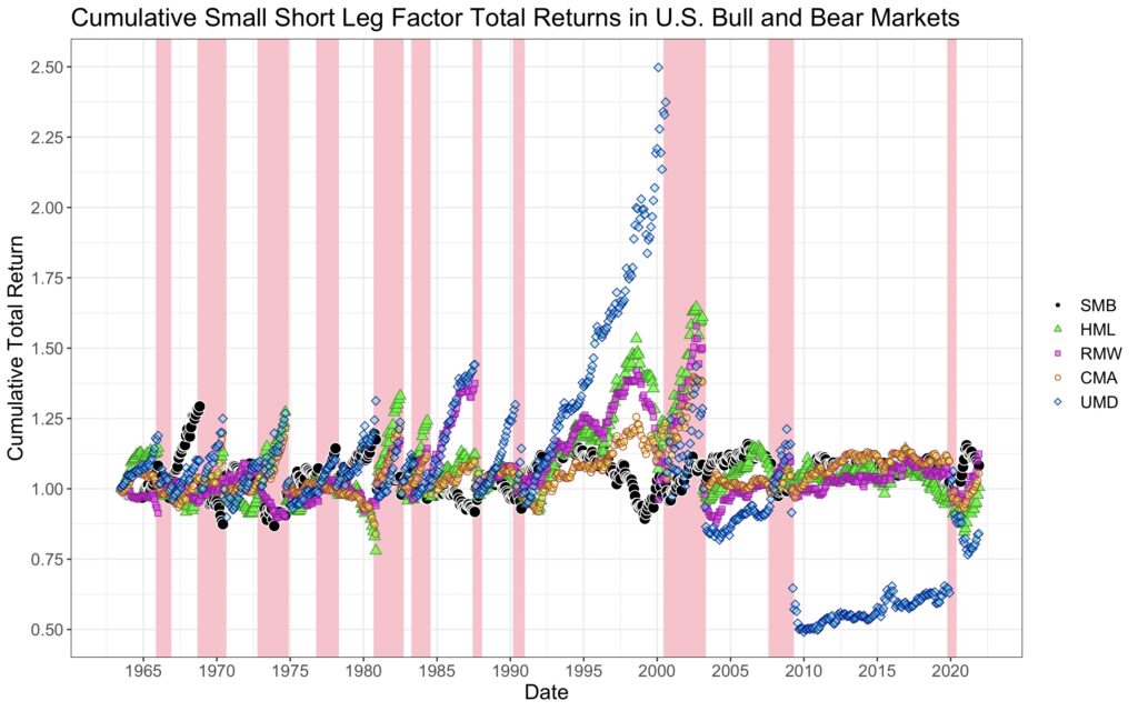
Similarly, in the next figure, we can observe the cumulative returns of the short leg of the factor returns. It is evident that bear market returns mainly originate from the short leg. Likewise, the momentum crash in the aftermath of the GFC is largely driven by the short leg.
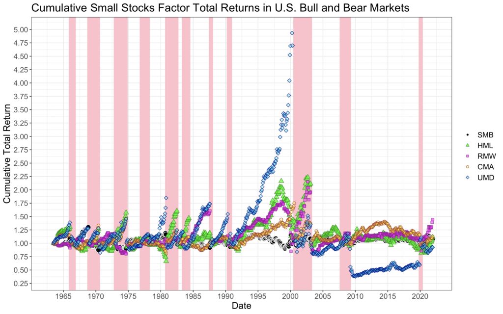
In addition, we plot the same figures separately for big and small stocks (see Appendix for the figures). Observations are relatively similar both in the big and small stock spaces.
Factor returns: a sum of long and short legs
Blitz, Baltussen, and van Vliet demonstrate in When Equity Factors Drop Their Shorts [3] how to separate the long and short leg returns of equity factors. They find that, on average, factors generate higher risk-adjusted returns (i.e., higher Sharpe ratios) in their long leg compared to the short leg, and that the long and short leg returns are highly correlated with each other. Their findings suggest that long-only factor investing or hedging long-only factors with the market portfolio can provide benefits over long-short factor investing, even if it theoretically captures only about half of the premia.
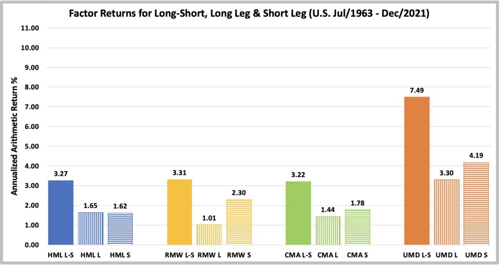
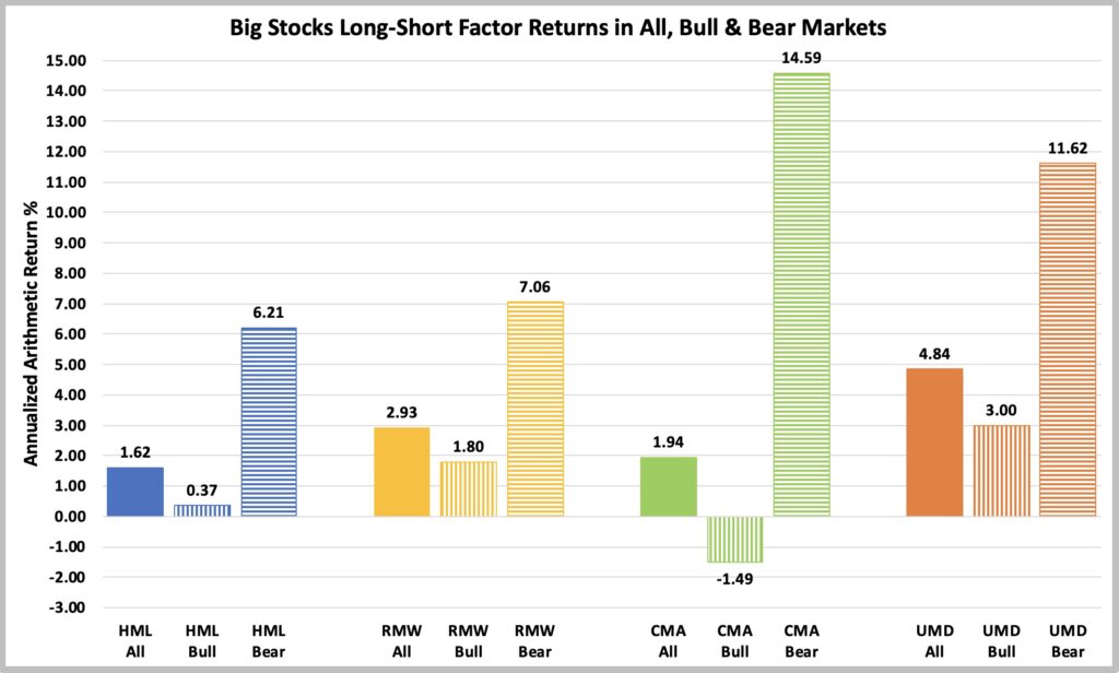
The figure below shows the factor premia in the form of long-short, long leg, and short leg returns. The long-short premia are calculated by summing the returns of the long and short legs. Generally, the premia are fairly evenly distributed between the long and short legs, with the exception of the profitability factor, where the return is largely driven by the short leg. The momentum factor exhibits the highest mean return by a wide margin, but this figure does not account for high turnover and trading costs associated with momentum strategies.
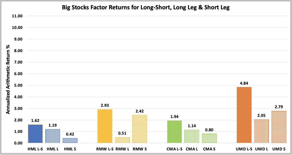
Next, we present the same analysis for the big stocks space.
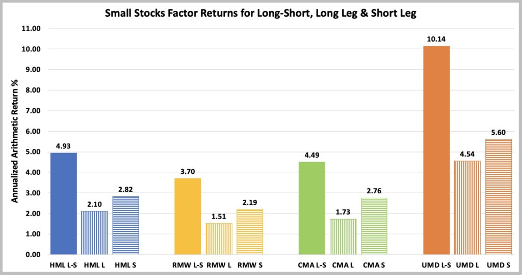
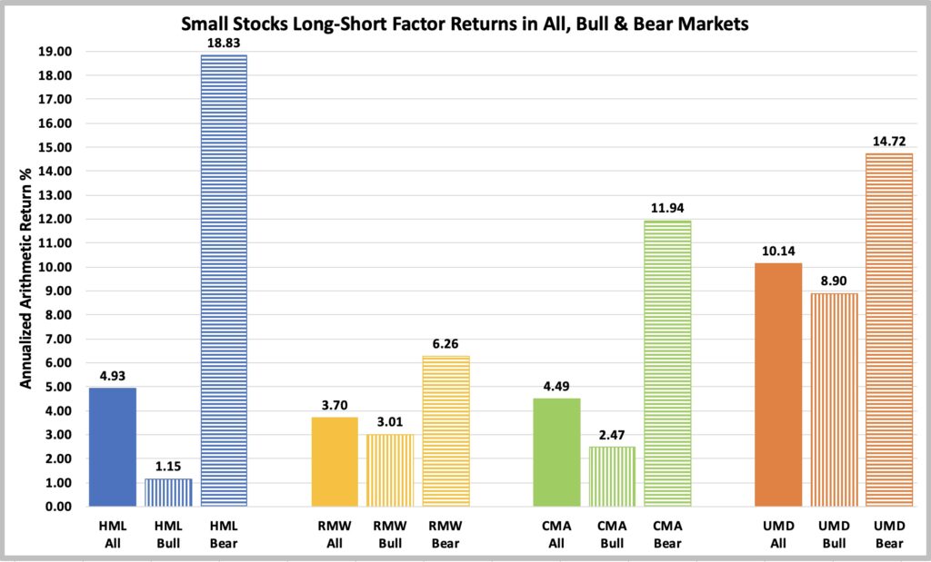
The small stocks space is shown below. Small stocks factor premia are on average much higher compared to big stocks premia, although trading costs can be assumed to be higher for small stocks.
Bear markets dominate factor premia
Geertsema & Lu, in their paper Where is the risk in risk factors? Evidence from the Vietnam war to the COVID-19 pandemic [1], show that factor premia are considerably higher during bear markets compared to bull markets. This finding can be somewhat surprising, as economic theory would suggest we should expect lower returns from assets that perform well in bad times (bear markets). Nevertheless, factors appear to deliver a meaningful premium in the long term and provide higher returns precisely when they are needed the most during bear markets.
Geertsema & Lu construct duration factors and find that duration can explain the high factor returns during bear markets. The intuition is that the required equity risk premium is time-varying and typically increases during bad times (bear markets). When the equity risk premium rises, future cash flows are discounted at a higher rate, which causes the present value of higher duration assets to decrease more than that of lower duration assets. For example, according to Geertsema & Lu, value stocks are consistently lower duration assets compared to growth stocks, which implies that the value factor benefits from an increase in the required equity risk premium. In fact, the authors demonstrate that when the factors are regressed against the duration factors they construct, bear market factor returns for value, profitability, investment, and momentum either vanish or decrease significantly, and in most cases become statistically insignificant.
Blitz, in his paper The Cross-Section of Factor Returns [4], also finds that factors have significantly higher returns during bear markets compared to bull markets. According to Blitz, this may be explained by mispricing building up during bull markets, leading to low factor returns, and mispricing being quickly corrected during bear markets, resulting in high returns. Blitz estimates that about half of the lower factor returns after 2004 compared to before 2004 are explained by the low frequency of bear markets. The market was in a bear market state 27% of the time before 2004 and only 9% of the time after 2004.
We show arithmetic factor mean returns in different states of the stock market in the figure below. The figure supports the results of Geertsema & Lu and Blitz, demonstrating that all factors except the size factor have delivered significantly higher mean returns during bear markets compared to bull markets. According to Geertsema & Lu, the size factor’s performance can be partly explained by financial constraint factors. This is reflected in the size factor’s tendency to show stronger performance in bull markets when financial constraints are typically lower. On the other hand, Blitz shows that the size factor has meaningful exposure to lagged market factor returns, indicating that the illiquidity of small stocks hides some of its market exposure. This suggests that the size premium can be explained by combining its exposure to both real-time and lagged market factor returns, and that its poor performance during bear markets can be attributed to its high exposure to the market factor.
We have 702 months in total, comprising 552 bull months and 150 bear months. For example, the mean return for value factor can be calculated: 3.27% = (552*0.76% + 150*12.52%)/702.

We can further decompose factor returns in bull and bear markets into long leg and short leg components. The next figure shows the mean returns for the long legs of these factors.
In this decomposition, bear markets are no longer the dominant source of returns. Only the long leg of the value and investment factors continues to show higher returns in bear markets compared to bull markets, though this difference is not nearly as significant as the difference observed with long-short factors.

The figure below shows that bear market returns primarily originate from the short leg of the factors. During bull markets, the short leg has produced minimal returns, especially when accounting for the costs associated with shorting.
The juiciest factor returns have occurred in the short leg during bear markets. However, as pointed out by Geertsema & Lu, it’s important to bear in mind that we do not account for trading costs, which can be particularly high for the short leg during bear markets due to elevated stock borrowing costs. On the other hand, even with long-only factor products, our historical data suggests that it is possible to outperform a benchmark portfolio without factor tilts, especially during bear markets.

We have run similar decompositions separately in the space of big and small stocks (see Appendix for the figures). Observations are relatively similar in both the big and small stocks spaces. Small value stocks have delivered particularly high returns during bear markets, and while the short leg still dominates, a healthy proportion of returns has also originated from the long leg.
These bear markets returns can be attributed to the spectacular run seen in the Dotcom bear market, right? Valuations of large, non-profitable growth stocks were extremely high, so it’s not surprising that small stocks, along with value and profitability factors, performed well during the ensuing bear market? Not really. If we remove the Dotcom bear market from our data (see Appendix for the figures), our conclusions remain largely the same. While small stocks do perform worse in bear markets and factor returns are somewhat lower compared to the original data, the overall pattern persists: factor returns are still highest in the short leg during bear markets. For the profitability factor, however, we observe that excluding the Dotcom bear market leads to higher mean returns during bull markets than in bear markets.
Correlations between factors
Blitz, Baltussen & van Vliet showed in When Equity Factors Drop Their Shorts [3] that the Sharpe ratios are higher for both individual factors and multifactor portfolios in the long legs of the factors compared to their short legs. This difference is reflected in the correlations between the factors.
Full sample
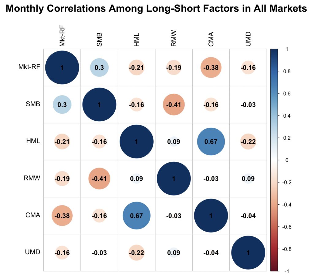
The figure below shows the monthly correlations between all long-short factors in our full data sample. The correlations between the value, profitability, investment, and momentum factors are close to zero, with the exception of the value and investment factors, which correlate heavily with each other. We can observe that these factors have a negative correlation with the market factor. Additionally, the size factor is positively correlated with the market factor.
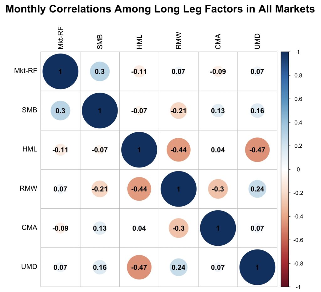
In the next figure, we can see the correlations between the long leg returns. The exception is the market factor, which is always presented in long-short format in our tests and figures.
We observe that the correlations between the value, profitability, investment, and momentum factors are now clearly lower compared to the long-short factors. Value and investment are no longer correlated, suggesting that their long-short correlation arises from the short leg. In fact, value even has strongly negative long leg correlations with profitability and momentum. Additionally, there are no longer any meaningful negative correlations between these factors and the market factor, suggesting that the negative correlations arise from the short leg.
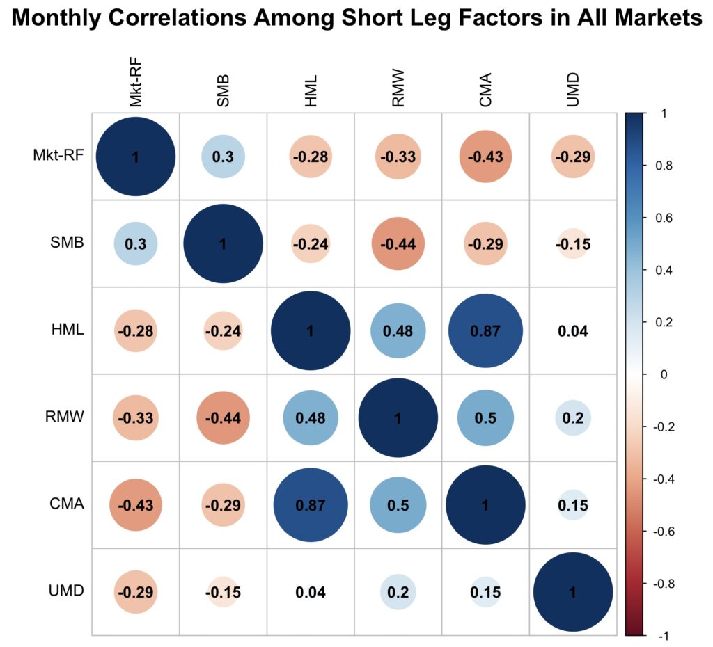
Finally, we show the correlations between the short leg returns. The value, profitability, and investment factors now correlate positively and heavily with each other. Additionally, these factors, along with the momentum factor, also correlate negatively with the market factor. The positive correlation between the value factor and the investment factor can be described as extremely high in the short leg.
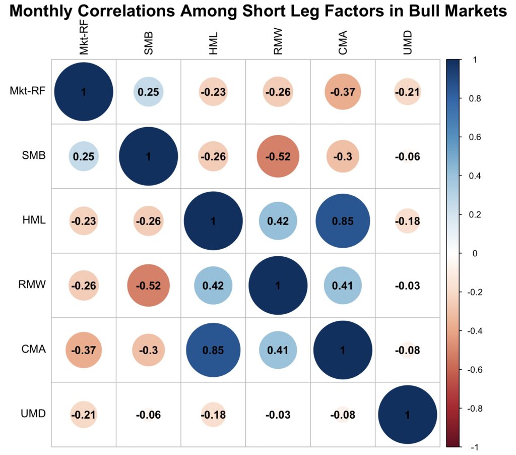
Bull markets
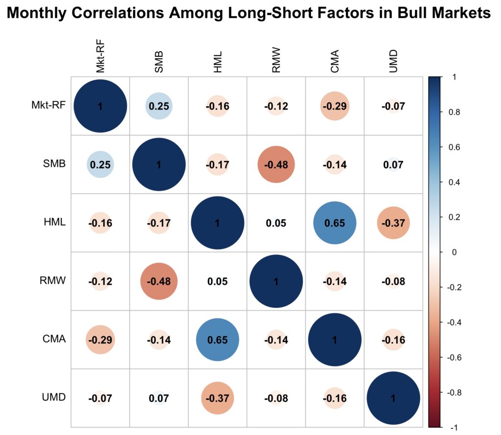
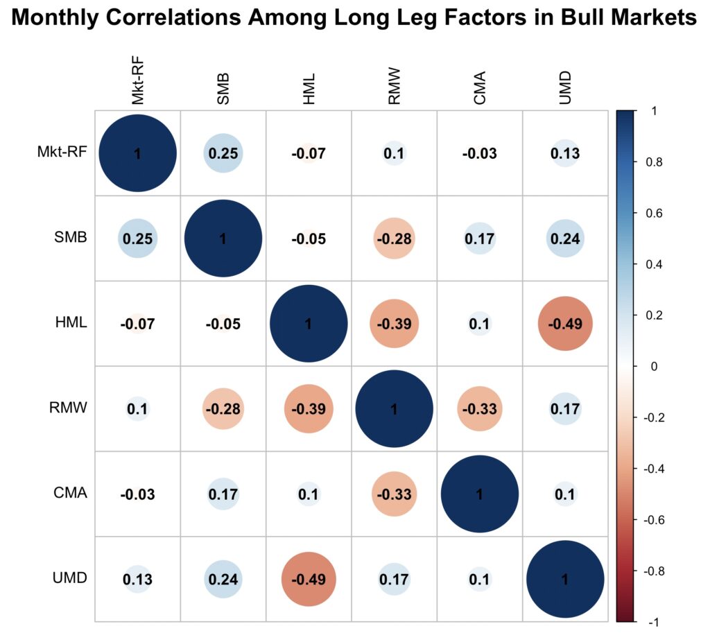
In the next three figures, we show the correlations for long-short, long leg, and short leg factors during bull markets. These correlations are fairly similar to the full sample correlations.
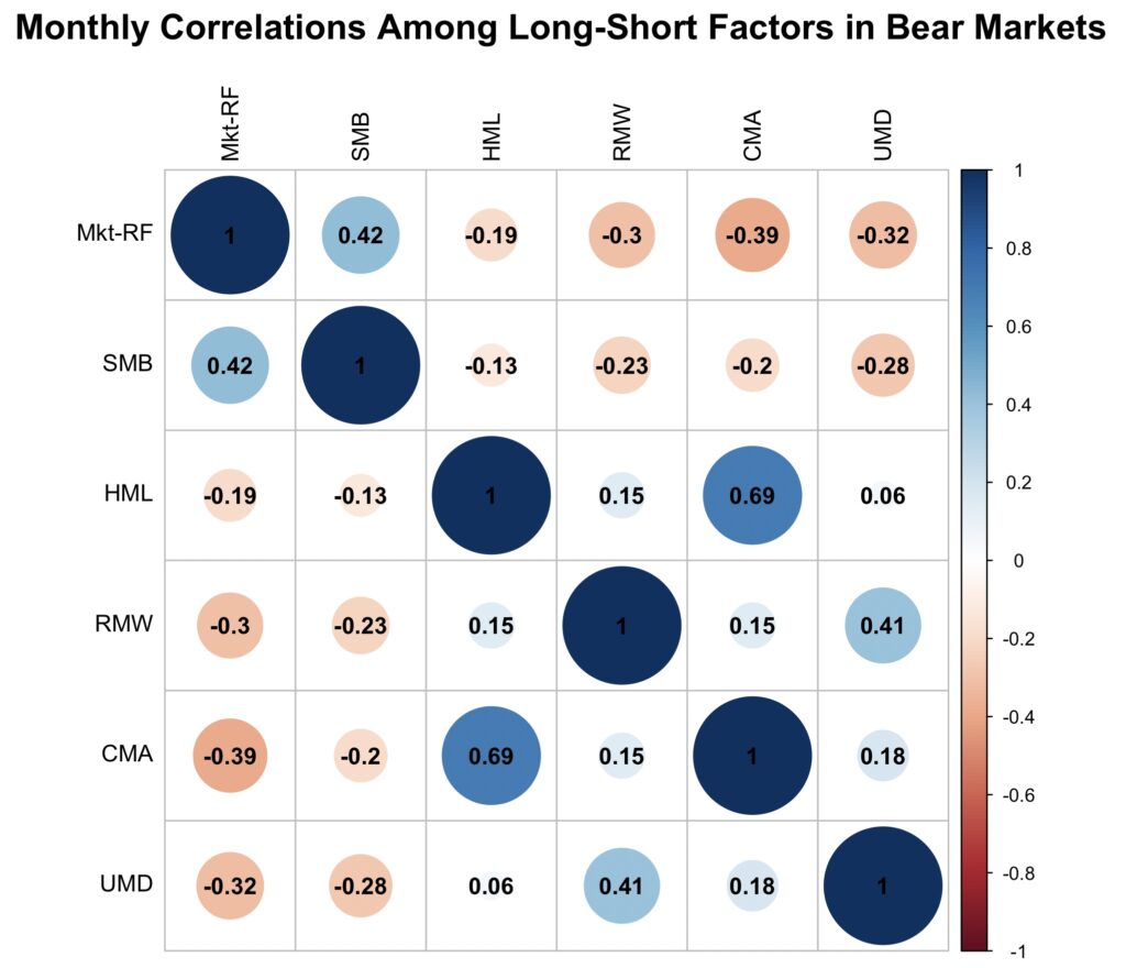
Bear markets
The next figure shows the long-short correlations during bear markets. There is a clear negative correlation between the market factor and the value, profitability, investment, and momentum factors. When the market moves down during bear markets, these factors tend to move up on average. Small stocks, however, have generally moved more in line with the market. We also see that the value, profitability, investment, and momentum factors exhibit relatively high positive correlations with each other during bear markets. As a result, these factors have not provided as much diversification benefit in a multifactor portfolio during bear markets as they do in bull markets.
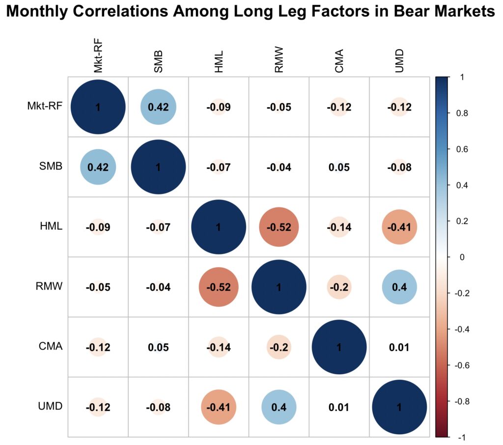
The figure below shows the correlations of long leg returns during bear markets. The long legs are not as negatively correlated with the market as the long-short factors were. However, the long legs of the value, profitability, investment, and momentum factors would constitute a highly diversified multifactor portfolio, as their correlations with each other are generally negative. However, only the value and investment factors exhibit meaningful positive mean returns in their long legs during bear markets.
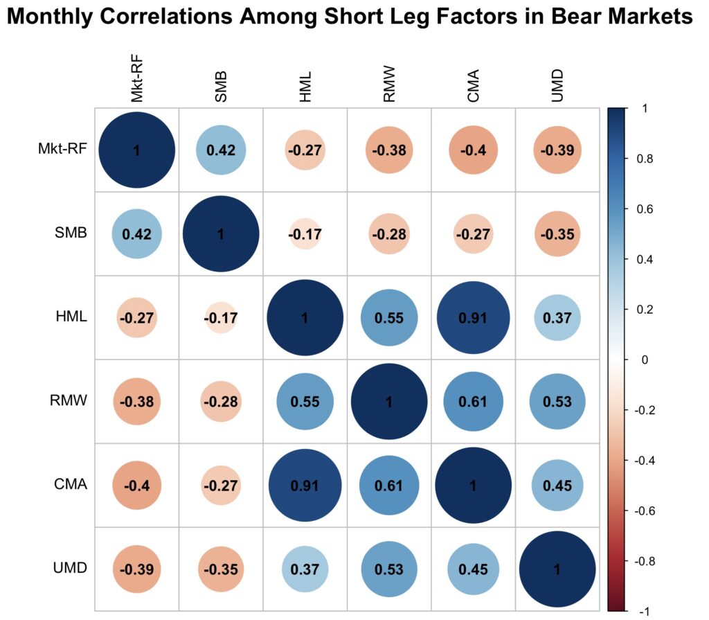
Finally, we show the correlations between the short leg returns during bear markets. The short legs of the value, profitability, investment, and momentum factors are now highly positively correlated with each other. This could be explained by a common factor exposure, such as the duration factor (as suggested by Geertsema & Lu), or by simultaneous mispricing correction, as suggested by Blitz. Whatever the cause, the effect is particularly strong in the short leg during bear markets. Additionally, we observe a particularly strong negative correlation between the market factor and the short legs of these four factors.
Conclusions
Equity factor premia can be decomposed into long and short leg premiums. While both legs contribute relatively evenly to the long-short mean return, the long leg typically provides higher risk-adjusted returns.
Small stocks provide higher factor premiums compared to big stocks, and momentum offers a higher premium compared to other tested factors. However, both the size and momentum factors suffer from higher implementation costs.
Decomposing factor returns into bull and bear market periods reveals that factor premiums for value, profitability, investment, and momentum have been significantly higher during bear markets. Further decomposition into long and short leg returns shows that the short leg has been particularly profitable during bear markets. However, this profitability may be partly paper returns as shorting in bear markets can be particularly costly.
High value, profitability, investment, and momentum factor returns in bear markets may be explained by a common factor, such as the duration factor, or by the correction of mispricing during bear markets. High bear market returns predominantly arise from the short leg of factor returns.
Lower-than-historical returns since 2004 for the value, profitability, investment, and momentum factors may be partly explained by the low frequency of bear markets during that period.
The size factor, which is correlated with financial constraint factors and has high and lagged exposure to market factor, has lower returns in bear markets compared to bull markets.
Correlation analysis demonstrates that the short leg returns for the value, profitability, investment, and momentum factors are strongly positively correlated with each other, particularly during bear markets. On the other hand, the short legs of these factors are strongly negatively correlated with the market. While the long leg has low or even negative correlations within a multifactor portfolio, it does not correlate negatively with the market factor during bear markets and therefore does not hedge market declines as efficiently as the short leg does.
Assessing factor returns using long-short factors across all equity market states may not reveal all relevant information, especially for long-only investors and those seeking protection from equity market drawdowns.
References
[1] Geertsema, P. & Lu, H. (2022). Where is the risk in risk factors? Evidence from the Vietnam war to the COVID-19 pandemic SSRN working paper, no. 3966127.
[2] Kenneth French data library
[3] Blitz D., Baltussen G. & van Vliet P. (2020). When Equity Factors Drop Their Shorts
[4] Blitz D. (2023). The Cross-Section of Factor Returns SSRN working paper, no. 4441376.
Appendix


Article by Markku Kurtti
Great stuff! PGIM speaks a little bit about the Time Varying Duration of the Value factor in the link below, but not to your depth:
https://www.pgimquantitativesolutions.com/white-paper/time-varying-duration-and-value-factor-correlation-interest-rates
Since you know factors so well, I would be interested to hear your thoughts on systematic variance vs Residual Volatility factor variance vs true idiosyncratic variance. I always struggle with the difference between Residual Volatility factor and true idiosyncratic risk. I would love to compare Res Vol vs true idio, and see if there are any surprising conclusions.
It might be hard for you to do this, since getting this granular generally requires you to have access to an actual factor model, which is expensive for an individual.
Thanks!
I am not sure how to distinguish between residual volatility factor and true idiosyncratic risk. To me, using a risk model and measuring residual volatility is a measure of idiosyncratic risk in the context of selected risk model (e.g. some known factor model). But it would be interesting to include also some volatility/beta based factors in my studies.
I’m also wondering if the short side of a factor could be used as a more cost efficient tail hedge, given its impressive convexity in bear markets…a retail investor likely couldn’t deploy a tail-hedge in this manner, but I wonder if a bank’s alternative risk premia team could construction something, or is all this strictly hypothetical. Something to think about!
Perhaps simply using long-short factors and potentially putting together a multifactor portfolio could serve as positive expected return strategy which has the tendency of doing well during bear markets.
Pingback: Weekend Reading - 1900-2024: The Optimal Equity Allocation & Equities In 2030: The Optimistic View Of The World.
Pingback: A Koala’s Guide to Factor Investing - Lazy Koala Investing