
We demonstrate how simple long-term volatility forecasts can be improved by incorporating the volatility of short-term volatility into forecasting models.
The theoretical framework for modelling volatility of short-term volatility, along with its role in long-term forecasts, will be outlined. Empirical tests will then illustrate the value of including volatility of volatility measures in practice.
A little bit of theory
In my earlier piece, The Kelly criterion in the presence of uncertainty about risk, we showed that long-term volatility depends on both the mean of short-term volatility and the volatility of short-term volatility, as expressed in the equation below.
This equation makes clear that forecasting long-term volatility using only mean short-term volatility—as in a simple linear regression—introduces bias and leads to a systematic underestimation. The bias arises from ignoring volatility of volatility.

We demonstrate the importance of accounting for volatility of volatility using empirical stock market data from Kenneth French [1]. Specifically, we use daily excess returns (Mkt – RF) from June 1952 through December 2024. We begin in June 1952, when U.S. stock markets changed to five trading days per week, averaging 252 trading days per year. Daily excess returns are annualized under the assumption of 252 trading days per year.
For our tests, we compute 21-day volatility of daily returns to represent monthly (short-term) volatility (252/12=21).
In the figure below, we group the empirical data into volatility quartiles. The circles (Theoretical Realized Vol) are calculated based on the equation introduced earlier. The figure shows that the equation predicts realized quartile volatility with high accuracy. In every case, realized quartile volatility exceeds the mean 21-day volatility, with the difference explained by the volatility of 21-day volatility.

Is short-term volatility forecastable?
We have shown that long-term volatility is determined by both mean short-term volatility and the volatility of short-term volatility. The natural next question is whether short-term volatility itself is forecastable.
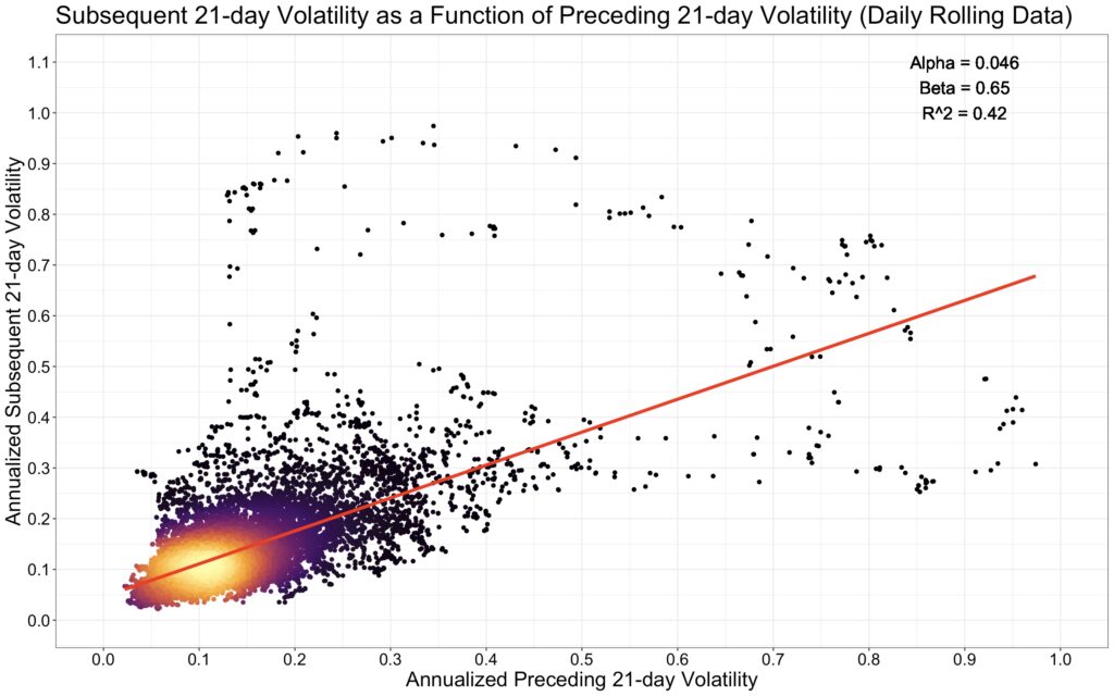
The simplest way to test this is with a linear regression. In our specification, illustrated in the figure below, subsequent 21-day volatility is the dependent variable and preceding 21-day volatility is the independent variable. We use a rolling 21-day window on daily data to maximize the amount of information.
The results suggest that short-term volatility is indeed somewhat predictable. In particular, volatility is mean-reverting: periods of low recent volatility tend to be followed by higher volatility, while periods of high volatility tend to be followed by lower volatility.
It is often said that using rolling (overlapping) data in regressions is problematic because it distorts statistical results. While it is true that rolling data inflates statistical significance, it can still be highly useful.
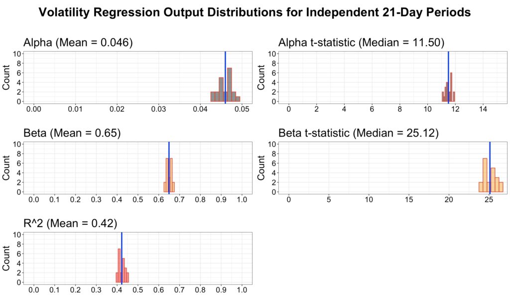
In the next figure, we use independent (non-overlapping) data across all 21 possible starting points. Compared to the regression with rolling data, the mean alpha, beta, and R-squared are essentially identical to those from the overlapping regression. In other words, rolling data removes the uncertainty associated with data timing and typically yields results that approximate the average of many independent regressions. I would go as far as to say that rolling data is the most hated useful thing in finance.
Modelling short-term mean volatility and volatility of volatility
Short-term volatility appears to be forecastable, but can we extend this to long-term volatility?
According to our equation, long-term volatility depends on two components: the average level of short-term volatility and the variability of short-term volatility itself. To forecast long-term volatility, we therefore need to forecast both of these short-term elements.
To uncover the functional form of this relationship, we apply a binned regression. While the original regression was quite noisy, binning the data filters out much of this noise and makes the underlying pattern clearer.
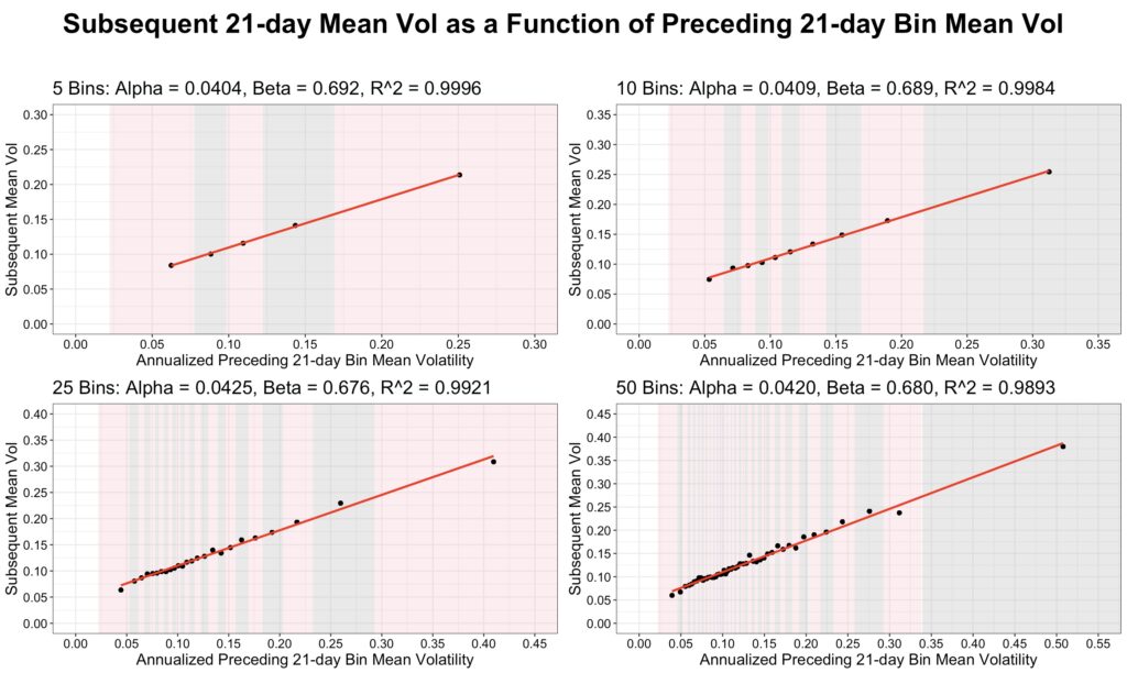
We create 5, 10, 25, and 50 bins based on 21-day volatility and show the corresponding fitted regression lines in the figure below. The relationship between mean preceding 21-day volatility and mean subsequent 21-day volatility is perfectly linear.
The standard (non-binned) regression can be interpreted as a binned regression in which the number of bins equals the total number of 21-day volatility samples. In other words, the non-binned regression represents an extreme case of binned regression for forecasting subsequent mean 21-day volatility. As the number of bins increases, the results of the binned regression converge to those of the non-binned regression, approaching the same outcome when the number of bins equals the number of samples.
Linear regression appears to work well for forecasting mean short-term volatility, but what about forecasting the volatility of short-term volatility?
Volatility of volatility is more challenging, because measuring the variability of volatility requires either more data or a partitioning of the existing data. We adopt a simple approach: for each 21-day period, we compute rolling 7-day volatilities, producing 15 overlapping samples, of which three are independent. To make these comparable with 21-day volatility, we normalize the 7-day volatility of volatility by multiplying by square root of 3 (since 21/7=3 and volatility scales as a square root).
We then use these 15 rolling 7-day volatility samples from the preceding 21 days as an estimate of preceding volatility of volatility.
Next, we bin the data based on this volatility of volatility measure and create 5, 10, 25, and 50 bins. The figure below shows that the relationship between subsequent mean 21-day volatility of volatility and preceding mean normalized 21-day volatility of 7-day volatility is approximately linear. This suggests that a simple linear regression can be used to forecast volatility of short-term volatility.

In-sample forecasting and volatility targeting
We can forecast both short-term mean volatility and the volatility of short-term volatility separately, and then combine these forecasts using our equation to obtain long-term volatility forecast. We next compare the performance of this combined approach with a simpler method that relies only on short-term mean volatility forecasting (a regression of subsequent 21-day volatility on preceding 21-day volatility).
While binned regression may be more robust to outliers, it requires choosing the number of bins, which introduces an additional modelling choice. For simplicity, we use standard (non-binned) regression to forecast short-term mean volatility. However, to forecast volatility of short-term volatility, we must rely on binned regression in order to obtain enough data to measure it reliably.
The only difference between the combined forecasting approach and the simple method is that the combined version incorporates the contribution from volatility of volatility. This can be viewed as a bias correction, since the simple method systematically underestimates long-term volatility by ignoring this component.
We use deliberately simple models, since our goal is to highlight the difference between including and excluding volatility of volatility in forecasts. We are not attempting to propose the best possible forecasting model, which would almost certainly require something more sophisticated than equally weighting the preceding 21-day data.
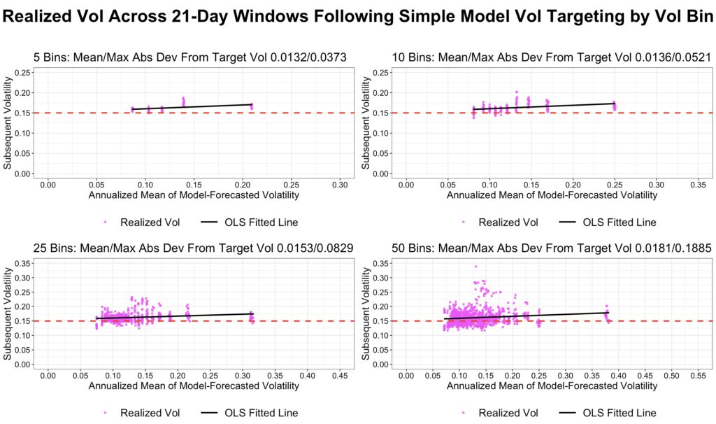
To test performance, we divide the data into 5, 10, 25, and 50 bins and apply both the combined and simple models to forecast bin volatility. For each bin, we calculate mean forecasted volatility and plot actual realized volatility against it. The regression is run separately for all 21 possible data timings, which is why each bin contains 21 samples. We then compute the OLS-fitted line for each of the four subfigures. In an ideal case, this line would have an alpha of zero, a beta of one, and an R-squared of one.
It is important to note that these are in-sample forecasts, meaning they incorporate information from the future. While such forecasts cannot be implemented in practice, they can still provide valuable insights into the relationships present in the data.
The first figure below uses the combined model, which incorporates volatility of volatility in addition to mean volatility. The results suggest that the model performs fairly well: alpha is close to zero, and beta is close to one.

The second figure below shows forecasts from the simple model, which does not account for volatility of volatility. Compared with the first figure, the simple model clearly underestimates realized bin volatility. This is evident from the regression line, where the beta is typically well above one, reflecting the fact that volatility of volatility tends to be higher at higher volatility levels. The alpha and R-squared values are quite similar to those of the combined model, suggesting that the main difference between the two approaches lies in the bias correction provided by including volatility of volatility.

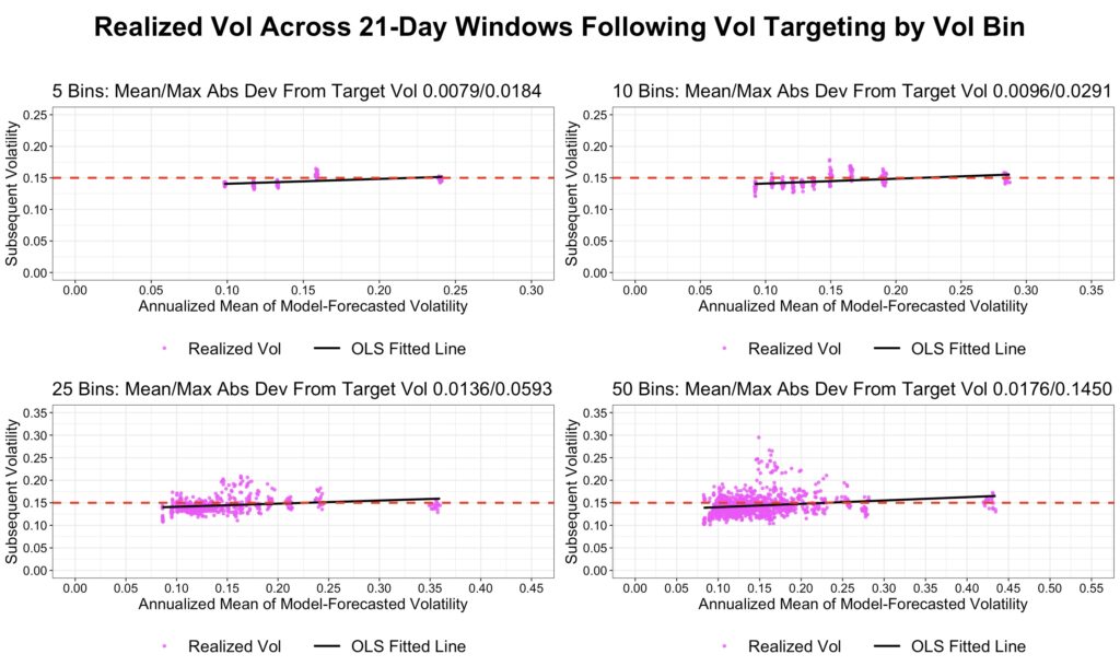
The next two figures show realized bin volatility when a constant target volatility of 15% is applied. Volatility targeting is implemented by adjusting leverage in proportion to the ratio of target volatility to forecasted volatility. We report both the mean and maximum absolute deviations of realized bin volatility from the 15% target.
The first figure, based on the combined model, shows that realized bin volatility tracks the target quite closely.
The second figure shows that the simple model underestimates volatility, causing realized volatility to systematically exceed the 15% target. This is evident from the mean and maximum absolute deviations, which are consistently larger than those of the combined model.
Out-of-sample volatility targeting
Out-of-sample models rely only on past data for their forecasts, providing a more realistic estimate of performance in real life.
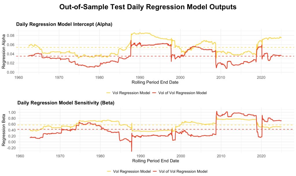
In our out-of-sample tests, we use 10 bins for the volatility of volatility model, while the mean volatility model—consistent with the in-sample tests—relies on non-binned regression. The models are estimated using the preceding ten years of data and then applied to forecast the next 21-day period. Based on realized preceding 21-day volatility and volatility of volatility, the leverage multiplier is adjusted each period to target a constant long-term volatility of 15%. The figures below show results from data utilizing rolling ten-year estimation windows, using the first possible data timing.
The figure below illustrates how the estimated models evolve over time. The yellow line represents the non-binned mean volatility regression model, while the red line shows the binned volatility of volatility regression model. Both models—particularly the volatility of volatility model—are highly sensitive to sudden shifts, such as the October 1987 crash entering or exiting the ten-year estimation window.
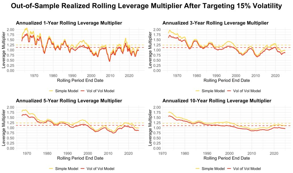
The next figure shows how the realized leverage multiplier evolves over time for rolling one-, three-, five-, and ten-year periods. The yellow line represents the multiplier from the simple model, which forecasts volatility using only the non-binned regression of mean short-term volatility. The red line represents the multiplier from the combined model, which estimates long-term variance as the sum of the squared mean short-term volatility from the simple model and the variance of short-term volatility from the binned model.
As expected, the leverage multiplier from the simple model is always higher than that from the combined model. This is because accounting for volatility of volatility increases long-term volatility, requiring a lower leverage multiplier to maintain the target volatility.
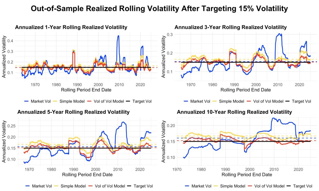
Finally, the next figure illustrates how well the models succeed in targeting long-term annualized volatility of 15%. Each panel shows the target volatility (black), realized market volatility (blue), realized volatility after targeting with the simple model (yellow), and realized volatility after targeting with the combined model (red).
Volatility targeting smooths out major market spikes and increases leverage during periods of low volatility. Realized volatility under the combined model is consistently lower than under the simple model. The bias correction from including volatility of volatility is best observed in the rolling ten-year window: the combined model oscillates symmetrically around the target, while the simple model almost always produces volatility above the target.
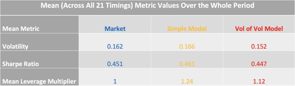
The table below summarizes key statistics over the full sample period from June 1962 to December 2024. The first ten years, beginning in June 1952, are excluded because they were used for model estimation. The values shown are averages across all 21 possible data timings.
The combined model (red) targets volatility much more accurately: its volatility targeting error is only 0.2 percentage points, compared with 1.6 percentage points for the simple model (yellow). Sharpe ratios are virtually identical across the market, the simple model, and the combined model. However, the average leverage multiplier is noticeably higher for the simple model (1.24) than for the combined model (1.12). This excess leverage is unintentional, arising solely from the failure to account for the effect of short-term volatility fluctuations on long-term volatility.
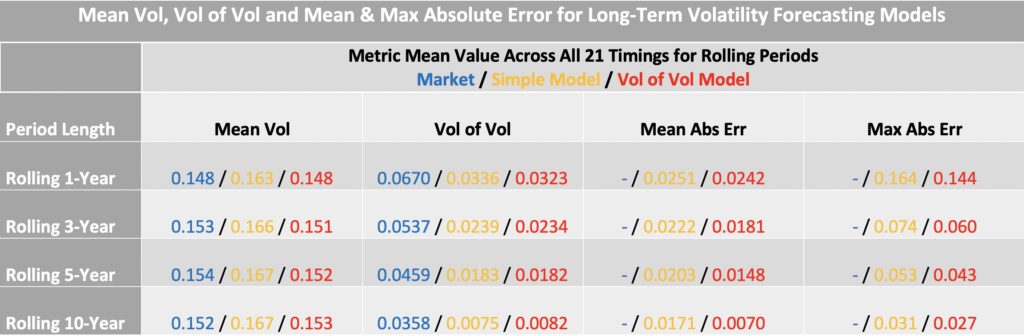
The next table summarizes statistics for different rolling periods. Across all horizons, the combined model (red) achieves more accurate volatility targeting than the simple model.
One of the main benefits of volatility targeting in general is the substantial reduction in volatility of volatility compared with the market. High volatility of volatility makes the use of leverage both difficult and risky; volatility targeting provides a framework that makes leverage feasible—or allows for higher levels of it. Many studies also find that volatility targeting increases the Sharpe ratio, though in our case the Sharpe ratio remains largely unchanged.
Incorporating volatility of volatility, as in the combined model, further reduces both the mean and maximum absolute error in realized volatility.
Conclusions
A simple regression that forecasts short-term volatility using only preceding realized short-term volatility will systematically underestimate long-term volatility. This is because long-term volatility is a function of two components: the mean of short-term volatility and the volatility of short-term volatility. Long-term variance can be expressed as the sum of the squared mean short-term volatility and the variance of short-term volatility.
Both components are forecastable. A simple regression effectively captures mean short-term volatility, while a binned regression can be used to forecast the volatility of short-term volatility. By combining these forecasts, we can correct the underestimation bias of the simple model and obtain accurate long-term volatility forecasts.
Using daily returns, we demonstrated that one-year to multi-year long-term volatility targeting can be improved by incorporating 21-day volatility of volatility into the model. The same approach applies to other time spans; for example, with 1-minute returns, a single day could be treated as long-term.
Our examples employ the simplest possible models to illustrate the role of volatility of short-term volatility. More sophisticated models could further improve long-term volatility forecasts.
References
[1] Kenneth French Data Library
Article by Markku Kurtti