A voting machine or a weighing machine?

“In the short run, the market is a voting machine but in the long run, it is a weighing machine” is attributed to Benjamin Graham. Another industry giant, John Bogle, categorized total stock market returns into two components: the fundamental return or investment return (dividend return plus earnings growth) and the speculative return (change in valuation). We can think of the fundamental return as the weighing property of the markets and the speculative return as the voting property.

While there is consensus that the stock market behaves as a voting machine in the short term, with monthly or yearly returns being dominated by valuation changes, the question arises: Does the market transform into a weighing machine in the long term? Are market returns dominated by dividend return and earnings growth when given enough time to average out the swings caused by valuation changes? These are the questions we delve into in this article.

We examine the extent to which valuation changes contribute to the real total return of the stock market over the long term, spanning up to forty-year periods. Our findings indicate that while fundamentals play a predominant role in determining the mean return, the voting machine property of the markets remains remarkably persistent and continues to dominate the variance of total returns even over forty-year time spans.

The enduring voting machine property in the markets implies that forecasting long-term total returns in the stock market requires a primary focus on predicting changes in valuation. Shiller’s Cyclically Adjusted P/E ratio (CAPE) is recognized for its ability to predict long-term total returns in historical (in-sample) data. Our demonstration reveals that the predictive strength of CAPE is entirely attributable to its capability to forecast changes in valuation. Additionally, we find that while valuation levels have varied substantially in the history, long-term real fundamental return has on average remained surprisingly constant in different valuation regimes.

Mean real stock market return and its constituents in the U.S.

We can decompose the real total return of the stock market into three components: 1) reinvested dividend return, 2) real earnings per share (EPS) growth, and 3) change in valuation. The sum of these three factors constitutes the real total return of the stock market over any desired time horizon.

We employ Shiller’s empirical monthly data [1] to assess the extent to which changes in valuation (Shiller CAPE) account for the real total return of the stock market. Our approach involves a linear regression model in which the dependent variable (LHS) is the real stock market total return, and the independent variable (RHS) is the change in valuation. According to our real total return decomposition, the intercept (the portion of real total returns not explained by valuation changes), i.e., the alpha, in the regression should be equivalent to the fundamental return (the sum of reinvested dividend return and real EPS growth).

A similar methodology was employed by Cliff Asness in his article The Long Run Is Lying to You [2]. Asness utilized a regression model, where he regressed the excess return of the stock market (LHS) against changes in valuation (Shiller CAPE) (RHS). Using rolling yearly returns, he found that changes in valuation explained the majority of the variance in excess returns. Using this model, Asness also estimated that the mean stock market excess return between 1950 and 2020 was approximately 1.3 percentage points lower when excluding the contribution from the increase in valuation. Asness argues that this methodology, excluding the contribution from valuation changes, offers a preferred approach for estimating expected returns. In our analysis, we use real total returns instead of excess returns and extend the analysis to rolling 5, 10, 20, and 40-year periods.

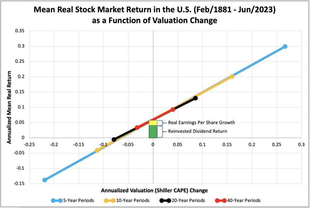
The figure below shows the result (regression lines) from our regression analysis combined with decomposition of the regression alpha to reinvested dividend return and real EPS growth components. Reinvested dividend return and real EPS growth are calculated for each rolling period from Shiller’s data, and we show the averages over the whole period. This figure is from the full period extending over 142 years from Feb 1881 to Jun 2023. More details about the regressions are provided in the next section.

In the figure we have the base (reinvested dividend return + real EPS growth) of the balance scale (the weighing machine) which elevates the beam (mean total return sensitivity to valuation change). The base of the balance scale represents the weighing machine property of the market and is approximately equal to the alpha of the regression. Beams represent the voting machine property of the market. The slope of the beam is the beta of the regression and each beam (for each time horizon) extends from the empirical minimum annualized valuation change to maximum change.

We can observe from the figure that valuation change dwarfs the real fundamental return as a determinant of the real total return. This is particularly true at shorter long-term horizons but remains surprisingly visible even at a 40-year horizon. While the real fundamental return determines the base rate (the higher, the better), valuation change sovereignly dominates the variability of the real total return.

Looking at the 40-year period range of returns, your initial impression may be that it is a weighing machine as the expected return is always positive and varies relatively little compared to shorter horizons. But valuation changes still explain 72.6% of the variability of the real total returns and if we consider the dispersion of terminal wealth, it is huge. The minimum real total return among 40-year periods is 3.1% (period ending in Jun 1932, with a -3.2% contribution from valuation change), and the maximum is 9.8% (period ending in Aug 1961, with a +3.5% contribution from valuation change). This translates to 14.6-fold difference (exp(40(0.098 – 0.031)) = 14.6) in terminal wealth. Notice that the annualized real fundamental returns for these two extreme periods are identical: 9.8% – 3.5% = 6.3% and 3.1% + 3.2% = 6.3%. The enormous difference in terminal wealths is entirely explained by changes in valuation. We discussed the effect of compounding and terminal wealth metrics in my earlier article Compounding materializes the importance of diversification.

The figure below represents the first half of the full period, where the voting property remains similarly dominant as in the entire duration. Real fundamental return is primarily driven by reinvested dividend return, with only a minor contribution from real EPS growth. We have dropped the 40-year period from the half-period tests because of lack of sufficient data.

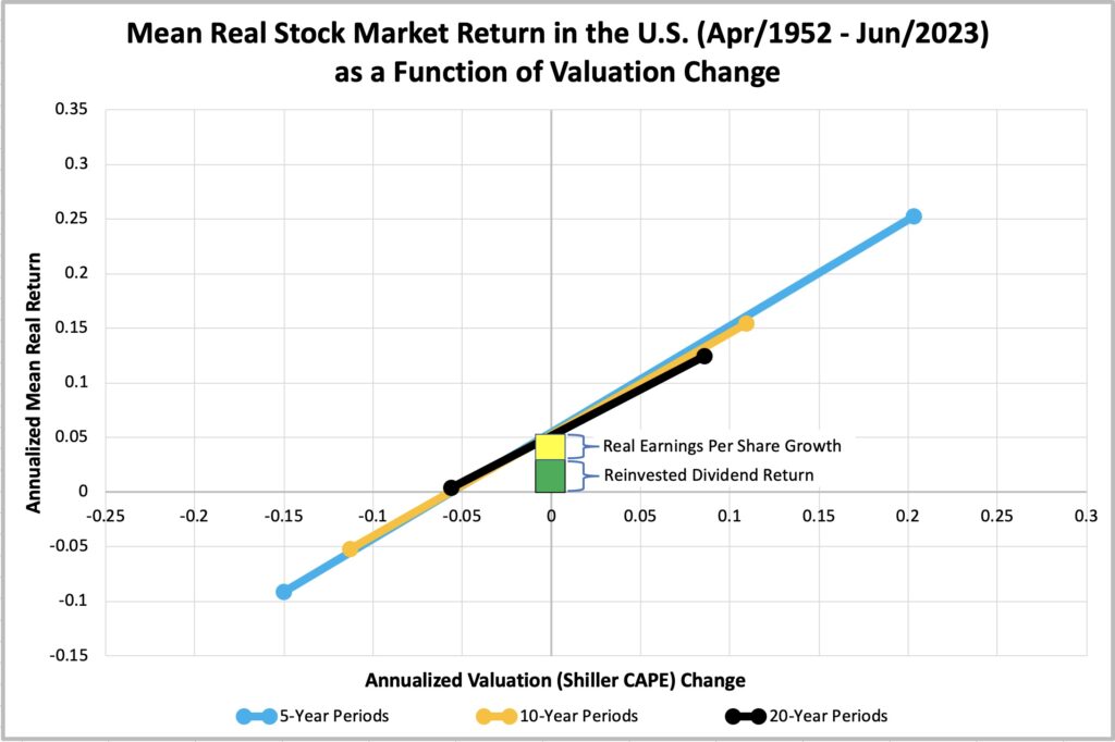
In the latter half of the period (figure below), we observe a greater contribution from real EPS growth to fundamental return, accompanied by a decrease in reinvested dividend returns compared to the first half. The magnitude of the fundamental return and the contribution of valuation changes to the total return remain relatively consistent across the first half, second half, and the full period.

Details of regression tests

An important aspect of the linear regression is that we need a linear relationship between the left-hand side (LHS) dependent variable we want to explain (annualized real total return) and the right-hand side (RHS) explanatory variable (annualized valuation change). To achieve the linearity, we need to use continuously compounded returns, i.e., log returns. With moderate annual returns, there is no practical difference between log returns and more commonly used yearly compounded returns. The difference becomes visible when the magnitude of returns is high. For example, if annualized log return is 6%, yearly compounded return is exp(0.06) – 1 = 6.18%. We can get back to log returns by calculating ln(1 + 0.0618) = 6%. But when log return is 50%, yearly compounded return is much higher at exp(0.5) – 1 = 64.9% or when log return is very low at -50%, yearly compounded return is considerably higher at exp(-0.5) – 1 = -39.3%. With log returns, it is also possible to have annualized return lower than -100%. E.g. -110% log return translates to exp(-1.1) – 1 = -66.7% yearly compounded return.

Furthermore, our decomposition formula is expressed as follows: real total return = reinvested dividend return + real EPS growth + valuation change. It’s important to note that this equation is mathematically exact only when employing continuously compounded returns (log returns).

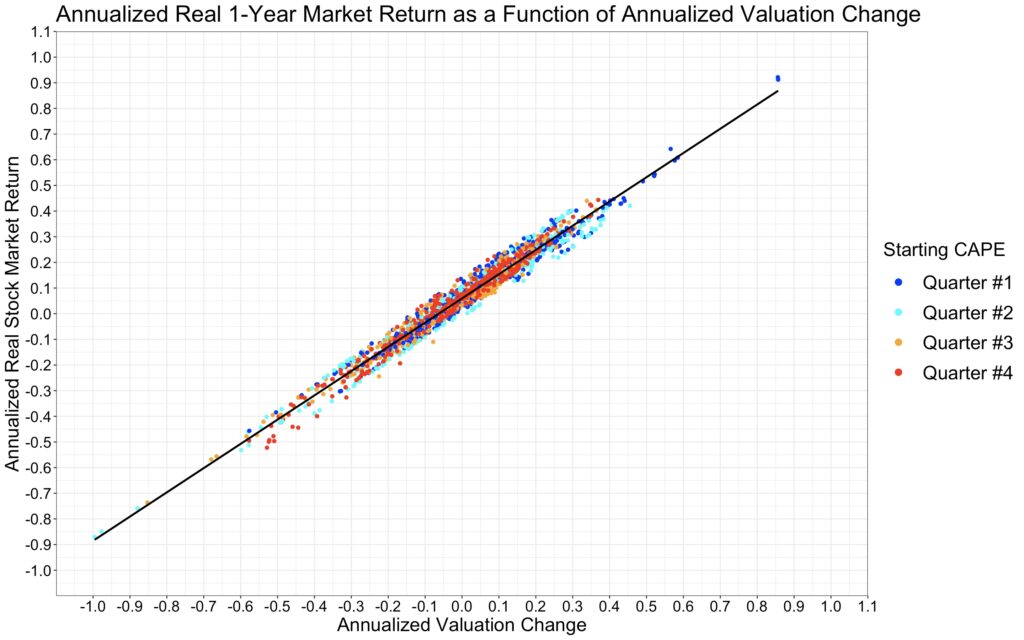
In the figure below, we illustrate the relationship between yearly real total returns (on the y-axis) and yearly valuation changes (on the x-axis), both expressed as log returns. The figure indicates that the relationship is precisely linear, with valuation change accounting for nearly all the variability in real total returns (R squared is 96.9%). We’ve incorporated color coding to represent the starting valuation quarters for the return data. Notably, there is no clear tendency related to the starting valuation in the yearly horizon.

The next figure combines 5, 10, 20 and 40-year period results. The relationship between annualized real total return and annualized valuation change is remarkably tight even at these long horizons. We also observe some correlation between starting valuation and valuation change: lower starting valuations tend to correspond to higher returns that have increased in valuation, while higher starting valuations tend to be associated with lower returns that have decreased in valuation.

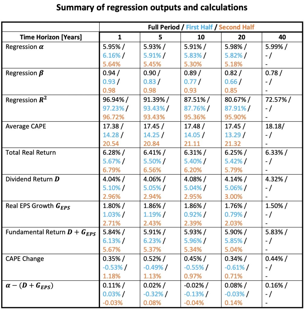
The table below summarizes the outputs from our regressions and calculations based on Shiller’s data. We present the results for the full period as well as the first and second halves of the data. In this context, we define real EPS growth as the growth from the end of the previous period to the end of the current period. An alternative approach would have been to calculate smoothed real EPS growth (which we later use in the next section) by determining the growth from the mean real EPS growth of the previous period to the mean real EPS growth of the current period. We choose the former method here because it provides more data for longer time horizons. On average, there is no difference between the methods when calculating the average real EPS growth over the entire dataset.

The last row of the table indicates that the intercept (alpha) of the regression closely aligns with the mean fundamental return (comprising reinvested dividend return + real EPS growth) calculated over all rolling periods per time horizon from Shiller’s data. This alignment is as expected, assuming that our real total return decomposition is correct and the tests are conducted properly.

As recommended by Asness, our best estimate of long-term returns should be derived from the alpha (the portion of real total returns not explained by valuation changes) of the regression, rather than relying on the realized return, which incorporates changes in valuations. Upon comparing the alpha and the realized real total return, we observe that the second half (the modern era) of the data (from Apr 1952 to Jun 2023) actually performed worse than the first half when changes in valuation are excluded. Consequently, the expected long-term real total return for the U.S. stock market, in the absence of valuation changes, appears to be closer to 5.5% than the often-cited (based on realized returns) 6.5% to 7% return.

The beta of the regression indicates the sensitivity of real total return to valuation changes. Overall, betas are consistently high, ranging from 0.94 (yearly horizon) to 0.78 (40-year horizon) for the entire period. Betas are slightly lower for the first period and higher for the second period. A beta of one would imply that real total return, on average, moves in tandem with valuation changes (i.e., a 1% change in valuation would on average correspond to a 1% move in real total return).

The R squared metric informs us about the proportion of variability (variance) in real total return that is explained by valuation changes. Surprisingly, given the length of our time horizons, R squared values are consistently high, ranging from 96.9% (yearly horizon) to 72.6% (40-year horizon) for the entire period. Similar to betas, R squared metrics are slightly lower for the first half and notably high for the second period. In summary, it appears that the modern era of real stock total returns (since Apr 1952) has been particularly sensitive and well-explained by changes in valuations.

Average CAPE indicates the market’s average expensiveness during a specified period. The second half has been almost 1.5 times more expensive compared to first half. Surprisingly, the alpha of the regression, representing the portion of total return not explained by valuation changes, has only been about 0.5 percentage points lower in the second period. This reveals a relatively small impact on fundamental return despite the significant difference in average valuation. The market seems to exhibit a degree of efficiency, as higher valuations expectedly lead to a lower dividend yield which is largely compensated by a rise in real EPS growth.

We have used rolling returns meaning that every possible start and end month is utilized in the data. Using rolling returns is beneficial especially when we have relatively few independent periods. Rolling data provides more information compared to utilizing only independent data points. But there is a well-known drawback in using rolling returns: standard errors of the regression will be downplayed and statistical significance will therefore be exaggerated. This problem can be tackled by using autocorrelation-robust standard errors, but there is also another way which we will use here.

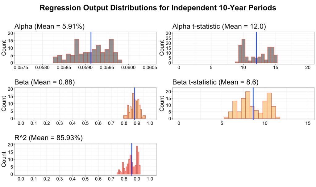
To get a reliable estimate of the statistical significance of the regression outputs and to test if the result if sensitive to timing of the data, we run the regression for all possible start months and utilize only independent (non-overlapping) data points. Using this method, we find that both alpha and beta of the regression are statistically extremely significant all the way up to 10-year horizon.

The figure below displays the distributions for independent 10-year periods, with 120 different timings for the data within each 10-year period. The results of the regression exhibit limited sensitivity to the timing of the test, and the coefficients are both economically and statistically highly significant. This is particularly noteworthy considering how small the sample size is (n = 14) for 10-year periods.

Rolling real stock market return and its constituents

Next, we will test our model as a function of time by factoring each rolling 10-year period into three return constituents, real fundamental return and finally showing the real total return for each period. To maximize the accuracy of our model, we utilize a 10-year horizon and align the real EPS growth metric with the earnings calculation of the Shiller CAPE. This is accomplished through a smoothed real EPS growth metric, calculated as the growth from the mean real EPS growth of the previous 10-year period to the mean real EPS growth of the current 10-year period.

If our model were perfect, three-factor regression alpha would be zero, all betas would equal one, and R squared would reach 100%. Upon running the regression, we obtain an alpha of -0.056%, a valuation change beta of 0.996, a dividend return beta of 1.037, and a real EPS growth beta of 0.997. The adjusted R squared is 99.99%. The mean absolute error, representing the mean absolute difference between real total return and the sum of the three factors, over all rolling periods is 0.093%, and the maximum absolute error is 0.33%. In summary, our three-factor model closely approximates a perfect decomposition of real total returns in 10-year horizon.

The chart below illustrates the rolling 10-year real total return breakdown over time. It’s evident at a glance that the significant fluctuations in real total return are driven by changes in valuation. Notably, reinvested dividend return was higher in the past, started decreasing in the nineties, and has consistently remained at a lower level through the new millennium. In contrast, fundamental return has maintained its normal levels despite the decline in dividend return. This resilience is attributed to the recent high real EPS growth. Various factors contribute to elevated EPS growth, including the shift from dividends to share repurchases. A portion of what was once dividend return has now transformed into real EPS growth. The figure highlights that dividend return has been the most reliable component of real total returns. The question remains whether real fundamental returns will become more volatile given the current higher average valuations and the dominance of real EPS growth as the primary determinant of the real fundamental return.

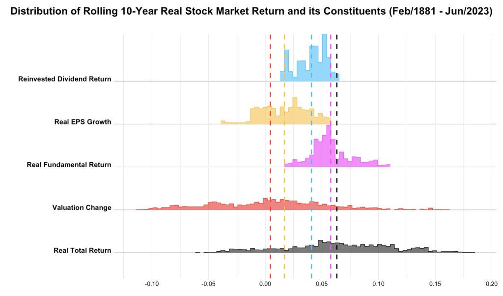
The following chart presents the distributions and means of the rolling 10-year real total return breakdown. It’s evident that the real fundamental return largely influences the mean of real total return, whereas valuation change plays a dominant role in shaping the variance of real total return.

Predicting long-term real stock market return

Having established that valuation changes dominate real total return variance even in the long run, this dominance becomes apparent when predicting stock market returns. Let’s consider two clairvoyants, one who can foresee real fundamental return for the next 10-year period and one who can foresee valuation changes.

The chart below depicts the real total return predictions in the form of a regression line for both clairvoyants. Basically, valuation changes are so dominant that the clairvoyant predicting fundamental return can’t foresee real total return at all, while the prediction from the clairvoyant specializing in valuation changes is nothing short of impressive. The color coding indicates the level of real fundamental return, and it’s evident from the valuation change clairvoyant’s prediction that if we could combine the talents of these two seers, we would achieve very close to 100% accuracy.

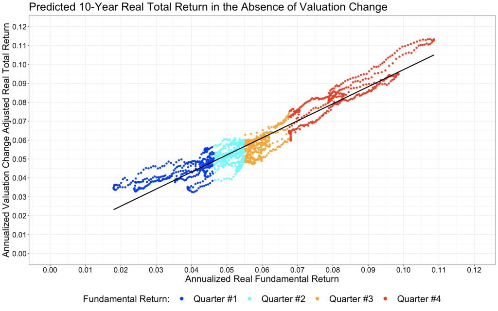
One might deduce that predicting real fundamental return has little value, but the matter is not quite as straightforward. If an investor is not capable or willing to predict valuation changes, the optimal strategy could be to assume that valuations will remain constant. We can approximate the prediction in the absence of valuation changes by subtracting the product of the valuation change beta (0.89) and the valuation change from the real total returns. This effectively flattens the regression line, bringing the sensitivity to valuation change (the beta) to zero. When we plot the result as a function of real fundamental return, as shown in the chart below, we observe that real fundamental return has a close to one-to-one mapping to the valuation change-adjusted real total return, as we should expect. This highlights that predicting real fundamental return still plays a role.

Shiller’s CAPE is renowned for its ability to forecast real total returns. Our next chart illustrates the source of this predictive capability. It becomes evident that the starting CAPE cannot forecast real fundamental returns for the upcoming 10-year period. Once again, we can interpret this as a sign of market efficiency, suggesting that, on average, valuations appear to be justified by the stock market’s ability to generate fundamental returns. On the other hand, we can observe that starting CAPE has clearly forecasted valuation changes for the next 10-year period.

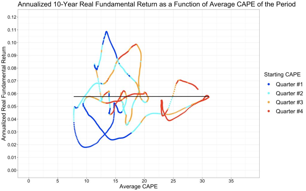
Instead of using starting valuation, we can depict the real fundamental return as a function of the average valuation of the period, as shown in the chart below. There is zero correlation between the average valuation level of the period and the real fundamental return during that period. It seems that valuations are perfectly justified by the average level of real fundamental returns that the market is capable of providing.

In the next chart, we observe that the valuation change predicted by the starting CAPE closely resembles the real total return predicted by the starting CAPE. To approximately align the regression line with the total return chart, we only need to mentally add the average real fundamental return (approximately 5.9%) to the valuation change chart.

So, should we conclude that starting CAPE has predictive power over the forthcoming 10-year real total returns? It certainly does in our tests, but these are all in-sample tests. It seems too bold a conclusion to draw for out-of-sample. When we have a predefined fixed sample, it will always have a minimum valuation and maximum valuation. Then, it is basically mechanistically guaranteed that the extreme valuations will mean revert towards the sample mean. But in out-of-sample tests, there are no fixed boundaries. The boundaries can move as can the mean valuation, as we saw when we compared the valuations in the first and second half of our data. If anything, it seems more plausible that valuations may revert towards a valuation level which can on average sustain a reasonable real fundamental return level rather than reverting to some arbitrary long-term average.

Conclusions

Ben Graham’s “In the short run, the market is a voting machine but in the long run, it is a weighing machine” seems to be partially true. The range of annualized outcomes does narrow as the time horizon lengthens, but valuation changes still explain the vast majority of the remaining 40-year return variability. In addition, when we consider terminal wealth after compounding, the effect of valuation changes is very large. Our takeaway is that the stock market never really loses its voting machine property when considering long horizons meaningful for most investors (5 to 40 years in our tests).

Valuation changes account for 96.9% (yearly horizon) to 72.6% (40-year horizon) of the variance in real total returns over the full period from Feb-1881 to Jun-2023. The explanatory power is slightly lower in the first half of the data and correspondingly higher in the second half.

While the realized return was higher in the second half, the return excluding valuation changes was lower. The estimated real total return of the U.S. stock market (based on rolling yearly returns) in the absence of valuation changes between Apr-1952 and Jun-2023 is 5.64%, compared to the realized 6.79%. In general, the fair estimate of the real U.S. stock market return in the absence of valuation changes is closer to 5.5% than the often-cited 6.5% to 7%.

In the second half of the data, valuations were, on average, considerably higher compared to the first half. Dividend return was considerably lower too, as expected when valuations are higher. Real EPS growth was considerably higher, almost enough to offset the lower dividend return. Overall, the fundamental return of the second half was only about 0.5 percentage points lower compared to the first half, which is a surprisingly small difference given the close to 1.5-fold difference in valuations. The market seems to have priced real fundamental returns efficiently. Similar efficiency is observed when we find no correlation between forthcoming 10-year real fundamental return and starting valuation (starting CAPE).

Valuation changes are so dominant that a clairvoyant capable of foreseeing real fundamental returns for the next 10-year period essentially struggles to predict real total returns. On the contrary, a clairvoyant specialized in valuation changes boasts an impressive track record. However, for an investor who is not capable or willing to predict valuation changes, assuming constant valuations may be a viable strategy. In such a scenario, the ability to predict real fundamental returns can add value.

The predictive power of Shiller CAPE over 10-year real total returns relies entirely on its ability to forecast valuation changes. However, it seems unlikely that there would be a constant average valuation towards which the CAPE would revert. Instead, if long-term valuations experience a gravitational pull, they may converge toward a prevailing level where a reasonable real fundamental return can be sustained.

References

[1] Robert Shiller Online Data

[2] Asness, C. S. (2021). The Long Run Is Lying to You

Article by Markku Kurtti