
Are stocks an inflation hedge? At least in the long run?
We find the answer to both questions is no. While fundamental returns—comprising dividend return and earnings growth—do help hedge inflation, valuation changes undermine this hedge. This holds true whether we examine yearly returns, ten-year returns, or anything in between.
Stocks do help protect our purchasing power from inflation, but not because they directly hedge against it. Instead, it is the risk premium that provides a buffer against inflation. However, this buffer is gradually eroded by inflation, meaning that higher inflation rates, on average, will reduce your real returns.
Yearly market return sensitivity to inflation level and change
We utilize U.S. inflation and stock market return data by Robert Shiller [1] after the end of the traditional gold standard (Gold Reserve Act of 1934) and convert the monthly data into quarterly data, spanning from Q1 1934 to Q3 2024.
Linear regression is used to demonstrate return sensitivity (beta) to both the inflation level (also referred to as “inflation” or “inflation rate”) and changes in the inflation level (inflation rate change). All returns, as well as the inflation level, are expressed in a continuously compounded (log return) format. Inflation rate change is measured as the percentage point change in the yearly inflation level, calculated as the difference between the inflation level of the ending year of the period and the inflation level of the year preceding the start of the period.
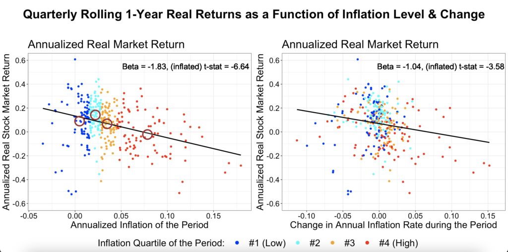
The yearly rolling data in the figure below provides a sample size of 360 observations. The average yearly inflation rate over all rolling periods is 3.5%. The data is overlapping, as we roll the yearly window with a granularity of one quarter. It is well known that overlapping data inflates statistical significance; however, it also reduces uncertainty related to the timing of the data. With non-overlapping data, one arbitrary timing must be chosen from many possible alternatives.
We observe that yearly real returns are highly sensitive particularly to the inflation level of the period and changes in the inflation rate during the period. On average, a one-percentage-point increase in the inflation level (i.e., the overall inflation rate for a given year) is associated with a 1.83-percentage-point decrease in real returns for that same year. Meanwhile, a one-percentage-point increase in the inflation rate change (i.e., the difference between the yearly inflation level at the start and end of the year) corresponds, on average, to a 1.04-percentage-point decline in real returns.
However, it is important to note that real returns exhibit significant variance that is not explained by inflation alone. Additionally, the relationship between real returns and the inflation level is not strictly linear. The optimal range appears to be in the second quartile of the inflation data, where real returns are relatively higher (as indicated by brown circles representing mean real returns for inflation quartiles).
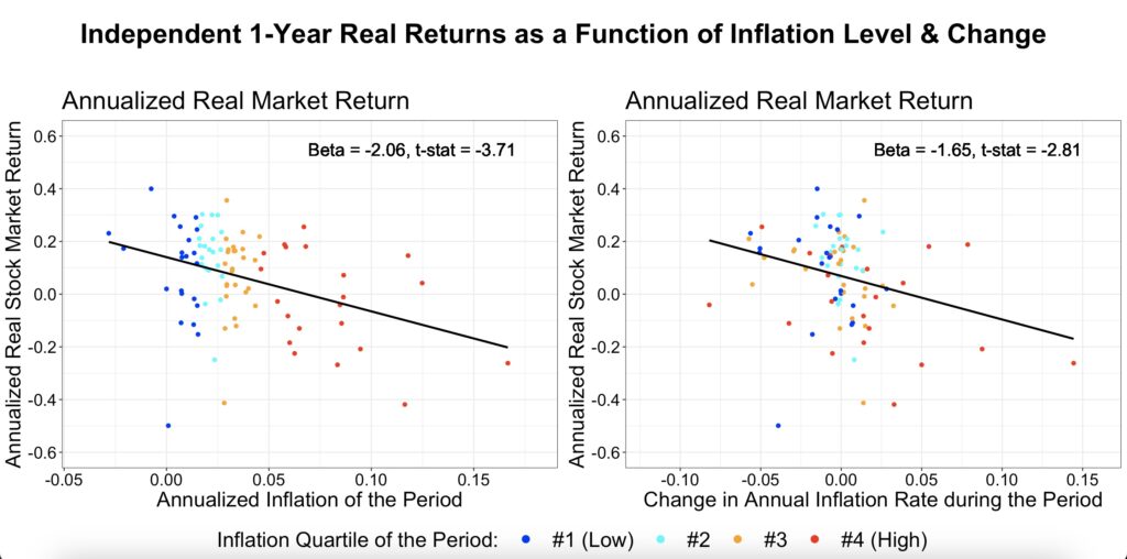
The next figure presents the same analysis but using non-overlapping yearly returns. The sample size is 90 years. While the betas differ from those in the rolling return regression, they remain within the same general range, at least for the inflation level. However, statistical significance is much lower in this case, as we are no longer reusing overlapping data to artificially inflate the t-statistic.
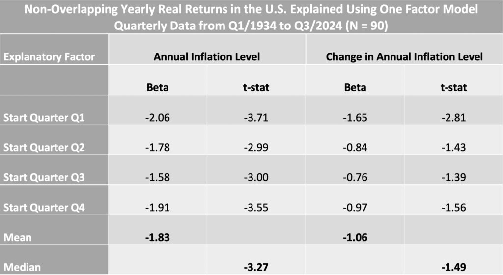
What about the different timings of the data? In the table below, we can see all four possible data timings. The first timing (start quarter Q1) corresponds to the non-overlapping data regression plot shown above.
What stands out is the surprisingly large variation in both the betas and t-statistics, particularly for the inflation rate change factor. The beta ranges from -0.76 to -1.65, while the t-statistic varies from -1.39 (not significant) to -2.81 (highly significant). This highlights how much statistical outcomes can depend on the arbitrary timing of the data—essentially, a matter of timing luck.
Another key observation is that the mean beta across all data timings is very close to the rolling data beta. This suggests that while rolling data (without adjusting for serial correlation) cannot be used to determine statistical significance, it may provide a more accurate beta estimate. This is because rolling data helps eliminate timing uncertainty, effectively filtering out timing noise.
In essence, data timing luck can be mitigated through the use of overlapping data, much like rebalance timing luck—as described by Corey Hoffstein [2]—can be mitigated by overlapping portfolios.
We calculate the median t-statistic to determine whether more than 50% of the data timings produce a statistically significant beta (with an absolute t-statistic greater than 1.96, the threshold for 5% significance). Alternatively, we could use methods like Newey-West standard errors, but this would require calibrating the standard error calculation by specifying the appropriate lag length to properly adjust for serial correlation.
However, our two factors (inflation level and inflation rate change) are not orthogonal, meaning they are correlated with each other. The correlation coefficient between the factors is 0.49 with yearly overlapping data. This correlation implies that using a single-factor model (by running separate regressions for both factors, as we did above) inflates both the absolute value of the beta and the t-statistic for each factor.
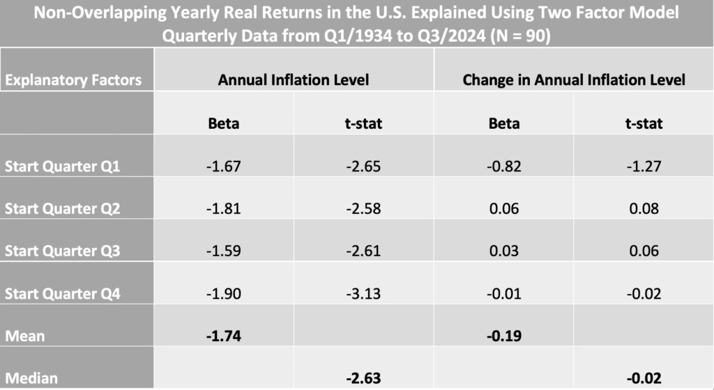
Instead of using just one factor to explain real returns, we can apply a two-factor model that incorporates both of our factors. The results of the two-factor model with different non-overlapping data timings are shown in the table below.
As expected, both the betas and t-statistics have been moderated compared to the one-factor model. It is clear that the inflation level is the dominant factor, remaining highly statistically significant across all four data timings. The inflation rate change factor, on the other hand, is entirely absent in three out of four timings, and even its largest beta of -0.82 is not statistically significant. After accounting for the correlation between the factors, only one remains.
Market return sensitivity to inflation level and change over different horizons
Okay, we’ve shown that real stock market returns are highly sensitive to the inflation rate. But as long-term investors, should we just wait for the market to show its true inflation-hedging capability over time? We will now show that increasing the time horizon will not help.
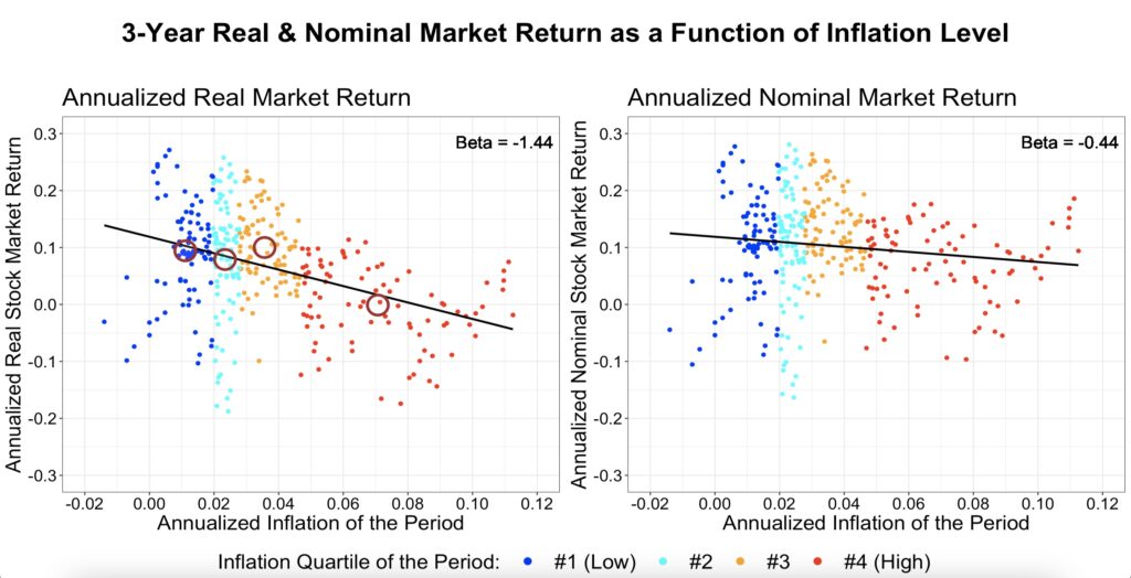
The figure below shows the medium-term, rolling 3-year horizon inflation sensitivity to both real and nominal stock market returns. If the stock market were an inflation hedge, we would expect real returns to be uncorrelated (with a zero beta) to the inflation level, and nominal returns to increase with a slope (beta) of one as a function of inflation level. However, as with yearly returns, we again observe that real returns are negatively associated with and highly sensitive to the inflation level. Even nominal returns show a negative inflation beta. This behavior is not what we would expect from a hedge.
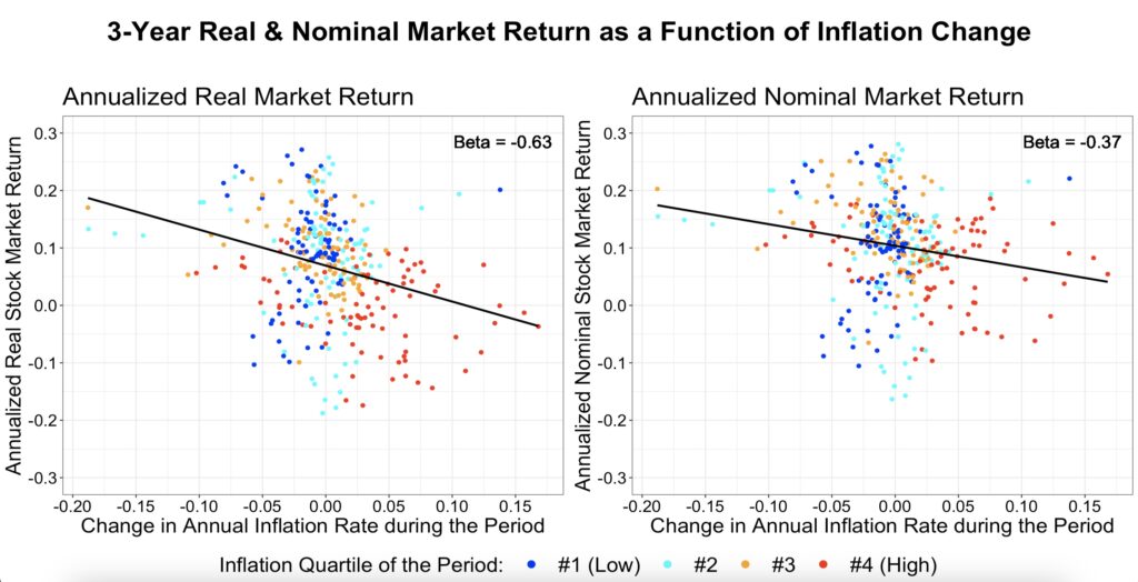
The next figure shows the sensitivity to changes in the inflation rate. There is a negative association between inflation rate increases and both real and nominal returns.
The two previous figures used a single-factor model, which we know will inflate the beta since our two factors are positively correlated. The next figure uses a two-factor model with overlapping data for the beta and non-overlapping data with all possible timings for the t-statistic. Both the beta and t-statistic are shown as a function of the investment time horizon.
In the long term, it is the nominal return inflation level beta, not the real return beta, that converges towards zero, though it does not quite reach it. The inflation level beta for real returns, however, converges towards minus one. In other words, in the long run, each additional percentage point increase in the inflation level translates, on average, to more than a one-percentage-point decrease in real returns. While betas for horizons longer than two years are not statistically significant, the historical evidence is clear: stocks have not hedged against inflation, even in the long run.
Furthermore, in the long run—at least historically, though not statistically significantly in our data—both the inflation rate and changes in the inflation rate during the period have been negatively associated with returns. The lines for real and nominal returns overlap for the inflation change beta (the inflation rate is captured by the inflation level factor in our two-factor model). Stocks have performed the worst under a regime of high and increasing inflation.

CAPE ratio change rate sensitivity to inflation level and change over different horizons
In my earlier article, A voting machine or a weighing machine?, we demonstrated how real stock market returns can be decomposed into the components of dividend return (reinvested dividends), real earnings growth, and valuation change. We found that valuation changes explained a surprisingly large proportion of return variance, even in the long run. Therefore, we have reason to believe that the relationship between inflation and returns may also be driven by valuation changes.
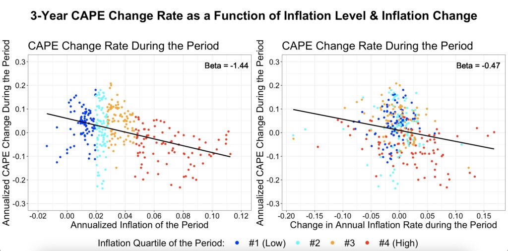
From the 3-year CAPE change rate figure below, we can see that it closely resembles the 3-year real return figures. The inflation level beta (-1.44) is exactly the same for both real returns and the CAPE change rate, while the inflation rate change beta is almost identical (-0.49 versus -0.47). The difference is that the real return scatter plots are shifted higher, as they include dividend returns and real earnings growth. However, the overall shape and slope of the scatter plots are strikingly similar.
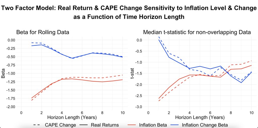
The two-factor model figure below displays the betas and t-statistics for the CAPE change rate.
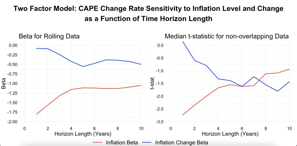
The similarity in both the betas and t-statistics between real returns and the CAPE change rate holds across any time horizon. In the figure below, we compare the real return betas and t-statistics with those of the CAPE change rate, and we find that both the betas and t-statistics are nearly identical.
It is the valuation changes component that drives the inflation sensitivity of stock market returns, and this holds true even over a decade-long horizon.
Dividend return sensitivity to inflation level and change over different horizons
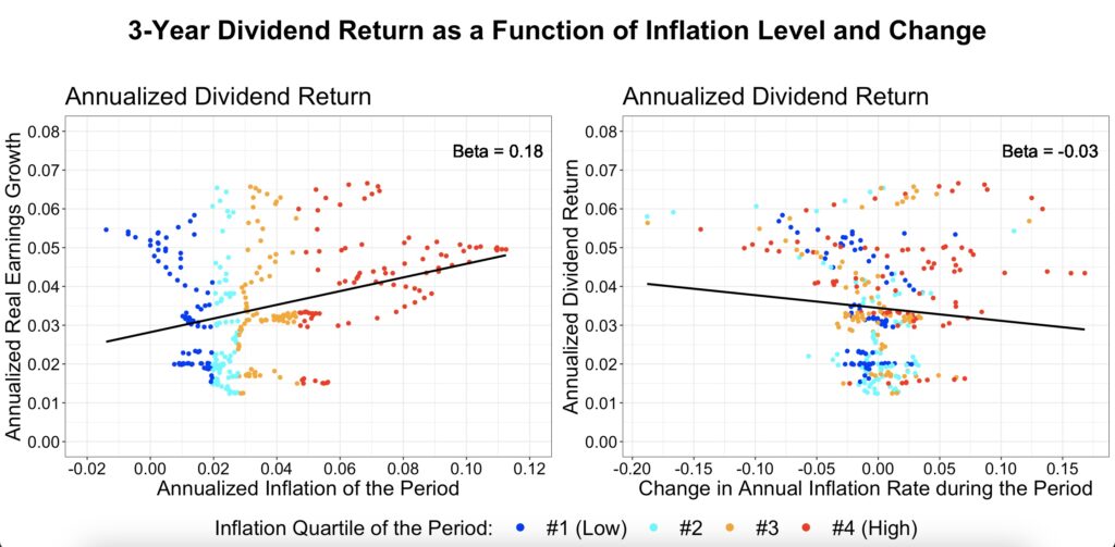
Dividend return is positively associated with the inflation rate, which makes sense because valuations decrease as a function of the inflation rate. As valuations decline (all else equal), dividend yield increases. However, dividends don’t appear to be affected much by changes in the inflation rate, as shown in the single-factor model figure below.
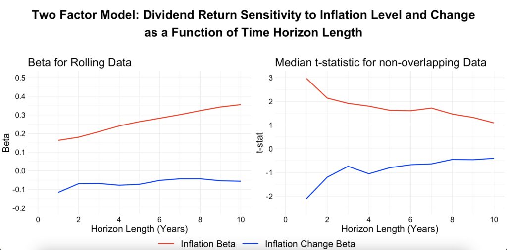
Using the two-factor model as a function of time suggests that dividend returns may become more strongly associated with the inflation level over longer horizons. It also indicates that changes in the inflation rate may have a small negative effect on dividend returns. This could potentially be interpreted as inflation decreasing valuations, which increases dividends, but at the same time, increasing inflation level might signal tough economic conditions for firms, encouraging them to retain earnings (therefore decreasing dividends). Both betas are statistically significant at the one-year horizon, as measured by the median t-stat across all data timings. The inflation level beta remains significant up to the three-year horizon.
Earnings growth sensitivity to inflation level and change over different horizons
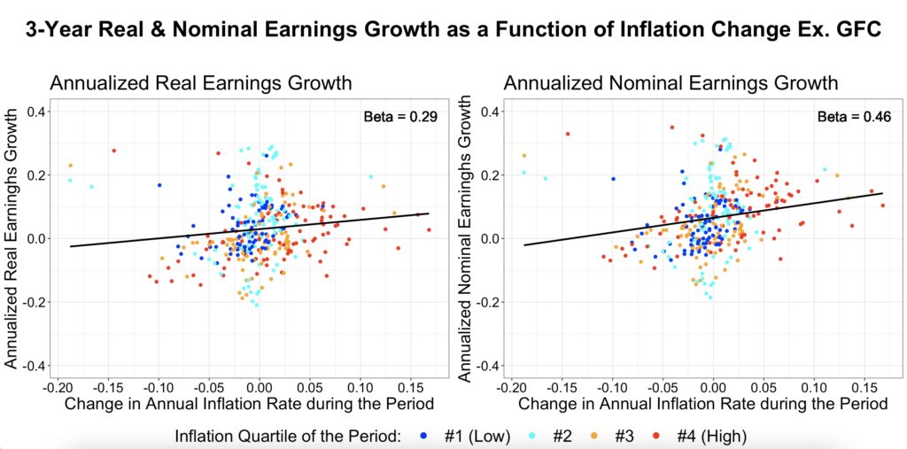
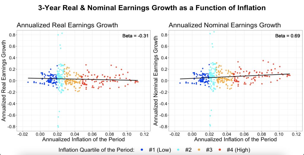
Earnings growth is where we would expect most of the magic to happen if stocks were a true inflation hedge. If firms were able to maintain constant real earnings growth regardless of the inflation level, then we would have a hedge. In this case, the inflation level beta would be zero for real earnings growth and one for nominal earnings growth. From the one-factor model figure below, we can see that there appears to be some hedging capability.
We are using data that excludes the global financial crisis period (Q4 2008 to Q4 2009) because earnings data during that time exhibited significant outlier changes, which were driven by the financial crisis rather than inflation. The figures with the full data can be found in the Appendix.
Note that we measure earnings growth ‘in real time’ over a given time horizon, meaning it is not synchronized with the Shiller CAPE valuation metric, which uses smoothed 10-year earnings growth.
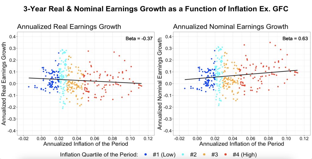
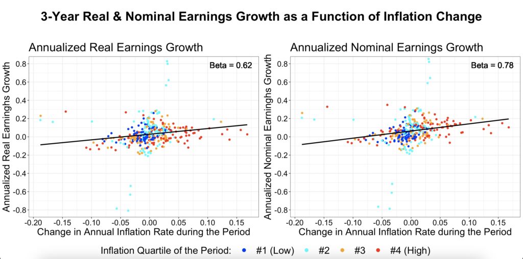
Earnings growth appears to be mildly positively associated with inflation rate changes.
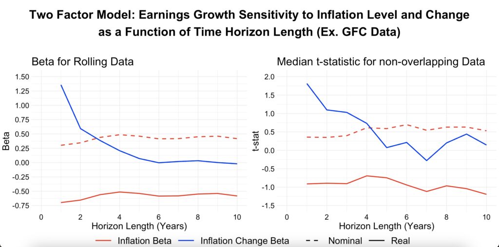
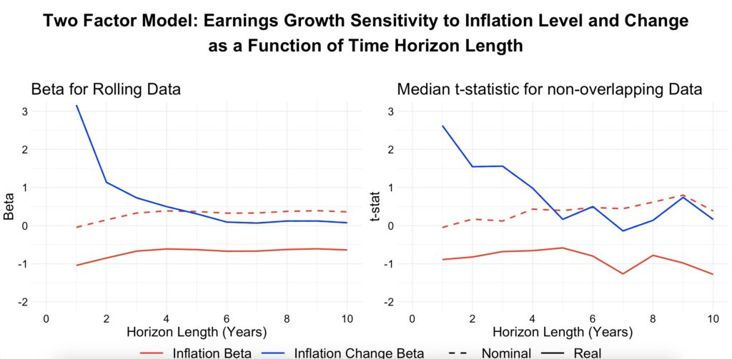
Using a two-factor model, we observe that in the long term, approximately half of the inflation level is hedged. In the short term, earnings growth appears to hedge against rising inflation, but this effect disappears over time. While none of these results are statistically significant, historical data shows that nominal earnings growth has been positively associated with the inflation level, helping to preserve purchasing power in the long run. Additionally, growing earnings appears to have provided a hedge against rising inflation in the short term.
Real Fundamental return sensitivity to inflation level and change over different horizons
Fundamental return is the sum of dividend return and earnings growth, representing the part of the return not explained by valuation changes.
If we used the same smoothed 10-year real earnings growth measure as the Shiller CAPE ratio, we would expect real total returns to equal the sum of the dividend return, real earnings growth rate, and CAPE ratio change rate. However, we have instead examined real-time earnings growth—rather than the smoothed version—to capture growth over a precise time horizon.
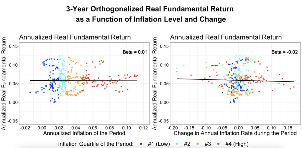
Rather than summing the three return components, real fundamental returns can also be determined by isolating them from real total returns. This involves removing the effect of valuation changes by first orthogonalizing real total returns with respect to the CAPE change rate. Specifically, we first determine the sensitivity (beta) of real total returns to the CAPE change rate and then subtract the CAPE change rate multiplied by this beta from the real total returns.
Orthogonalized real total return effectively represents the real return excluding valuation changes, making it the real fundamental return. This real fundamental return is now aligned with the smoothed real earnings growth measure used by the Shiller CAPE ratio. It can then be regressed against the inflation level and changes in inflation to determine its sensitivity to inflation.
Using the one-factor model, the figures below suggest that, historically, fundamental returns have had the ability to hedge inflation. Real fundamental returns appear completely indifferent to both the inflation level and changes in the inflation rate. Fundamental returns are crucial because, in the very long run, the impact of valuation changes diminishes, leaving only fundamental returns.
The two-factor model shows that, historically, fundamental returns have hedged inflation in both the short and long term.
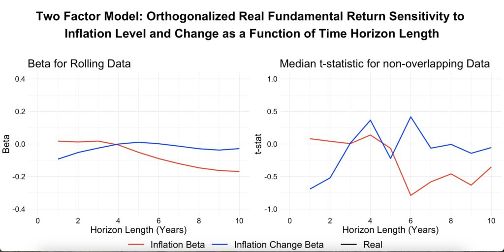
Based on our results, it appears that fundamental returns (dividend return + earnings growth) have historically been a fairly effective inflation hedge. However, decreasing valuations have dampened returns in high inflation environments. It’s important to note that decreasing valuations are necessary to increase dividend returns, which, in turn, contribute to higher fundamental returns. In high inflation environments, lower valuations are essential to preserve a healthy expected (very long-term) equity risk premium.
When we combine both the effects of fundamental returns and valuation changes, we arrive at total stock market returns. These returns have not acted as an inflation hedge, but rather as a buffer against inflation, provided by the equity risk premium. This buffer has been large enough to help preserve at least some purchasing power during inflationary periods, offering protection through the equity risk premium rather than through direct inflation hedging.
Conclusions
Historically, stocks have not acted as a hedge against inflation. Instead, they have provided a healthy risk premium, which has served as a buffer against inflation. On average, inflation has eroded that buffer, with higher inflation levels leading to lower real returns.
Stocks have shown high sensitivity to inflation rates. The inflation rate beta for real stock market returns has been around -1.75 using yearly data, and approximately -1.25 over longer horizons, up to ten years. The beta for yearly and two-year data is statistically significant for most data timings, whereas the betas for longer horizons are not. Increasing inflation rates have also been mildly negatively associated with real returns, with a beta of about -0.5 across time horizons from four to ten years. However, this relationship is totally absent at short horizons and not statistically significant at any tested horizon.
The stock market’s sensitivity to inflation is almost entirely explained by valuation changes, which are nearly identical in sensitivity to inflation compared to real stock market returns.
Real fundamental returns, comprising reinvested dividend returns and real earnings growth, have been largely indifferent to both the inflation level and changes in the inflation rate. Real fundamental returns have played their role in hedging inflation.
When we combine real fundamental returns with valuation changes, we obtain real stock market returns. Valuation changes—highly sensitive to inflation and negatively associated with it—dominate real return variance, resulting in real stock market returns that are also highly sensitive to and negatively correlated with inflation. This holds true in both the short and long term.
References
[1] Robert Shiller Online Data
[2] Corey Hoffstein Quantifying Timing Luck
Appendix
Earnings growth figures utilizing full data (GFC not excluded):
Edit history
24-Mar-2025:
Inflation rate change had accidentally one year offset in my data. This was fixed, which resulted in higher correlation between inflation level and inflation rate change factors. After the fix, inflation rate change became less significant, essentially non-existent at least in shorter horizons. Also, real fundamental return analysis was changed to be based on orthogonalized real returns (orthogonalization with CAPE change rate).
Article by Markku Kurtti
Pingback: On inflation and stock returns - MacroTrader.io