Some portfolio construction heuristics

Constructing a high Sharpe ratio portfolio, paired with sensible leverage, is the key to achieving meaningful returns with tolerable risk.

We will make some simplifying assumptions to build intuition, derive a set of formulas with accompanying figures, and run a simple simulation to demonstrate what is required to construct and monetize a high Sharpe ratio portfolio. Building such a portfolio requires effective diversification, which primarily means achieving low correlations among portfolio constituents. If alpha is present, low correlation and high Sharpe ratio can be achieved by hedging factor exposures. Monetizing the benefits of a high Sharpe ratio portfolio requires leverage. A large number of constituents with low average correlation, combined with leverage, is the key to success—but it also increases correlation risk.

Revisiting capital market parabola

In my earlier article, The Kelly criterion, capital market parabola & the almighty Sharpe ratio, we introduced the concept of compounding process capacity as an analogy to Shannon’s information channel capacity. In the same article, we used the figure below to illustrate the central role of the Sharpe ratio in determining both compounding process capacity (the maximum mean geometric excess return) and the capital market parabola (or capital allocation parabola), which serves as the geometric counterpart to the arithmetic capital market line (or capital allocation line).

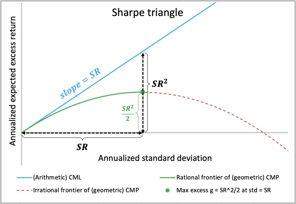
It is well known and proven that Shannon’s information channel capacity, or the Shannon limit, sets the upper bound for error-free data transfer rates in digital communications. But how well does compounding process capacity hold up empirically?

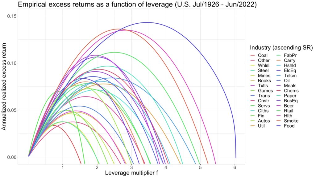
We can use daily U.S. industry returns from Kenneth French’s data library [1] to plot the annualized mean geometric (logarithmic) excess return for each industry as a function of the leverage multiplier (assuming lending and borrowing at the monthly T-bill rate). This is illustrated in the figure below.

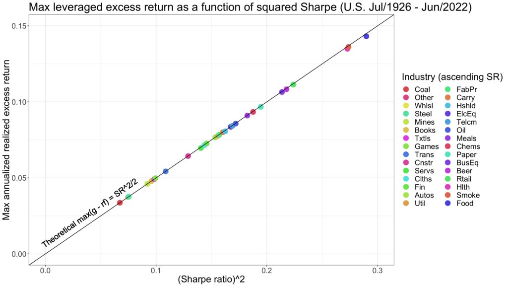
The formula for compounding process capacity states that the maximum attainable annualized mean geometric excess return — the Shannon limit — is exactly half of the annualized Sharpe ratio squared. The figure below demonstrates that compounding process capacity holds empirically.

We demonstrate below how the maximum-ratio combining [2], well known method in telecommunications, can be applied to derive equations for uncorrelated portfolio constituents. Our derivations align with Ed Thorp’s results (see equations 8.1 and 8.2 in The Kelly criterion in blackjack, sports betting and the stock market [3]). Additionally, the formula for optimal variance allocation as a function of squared Sharpe ratios matches that derived by Giuseppe Paleologo in Advanced Portfolio Management: A Quant’s Guide for Fundamental Investors [4]. We go a step further by deriving a formula for the Sharpe-optimal factor hedge ratio.

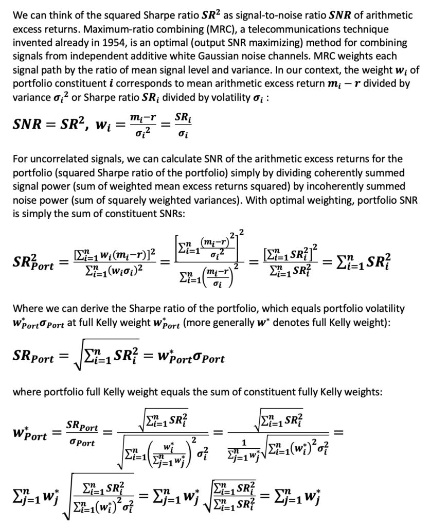
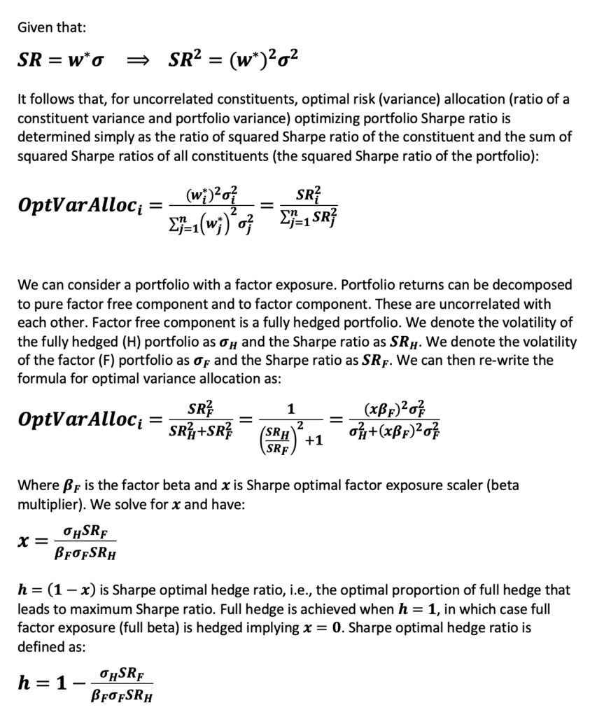
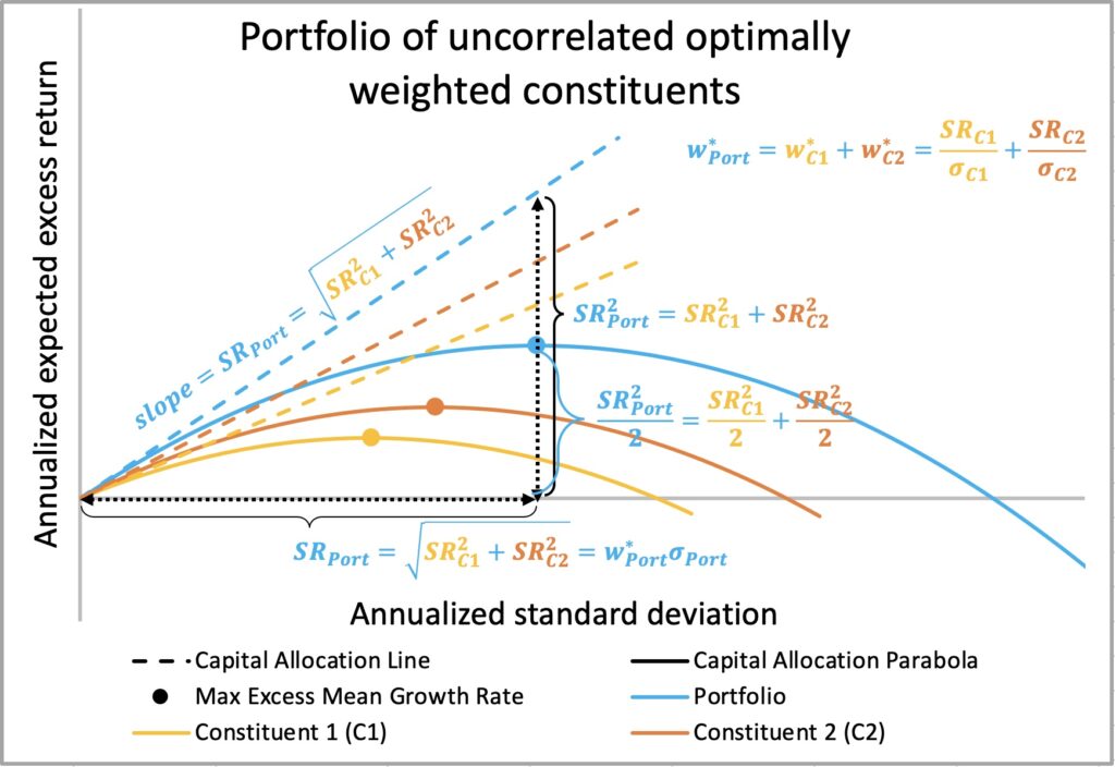
Using the formulas derived above, we can illustrate a Sharpe triangle for multiple uncorrelated assets, as shown below. The compounding process capacity of an optimally weighted portfolio is the sum of the capacities of its constituents, and the full Kelly weight is the sum of the constituent Kelly weights. At full Kelly weight, the portfolio’s Sharpe ratio equals its volatility, meaning the squared Sharpe ratio equals the portfolio variance. The sum of uncorrelated constituent variances (squared Sharpe ratios) gives the total portfolio variance. Thus, the Sharpe-optimal variance allocation for a constituent equals its squared Sharpe ratio divided by the sum of squared Sharpe ratios for the entire portfolio.

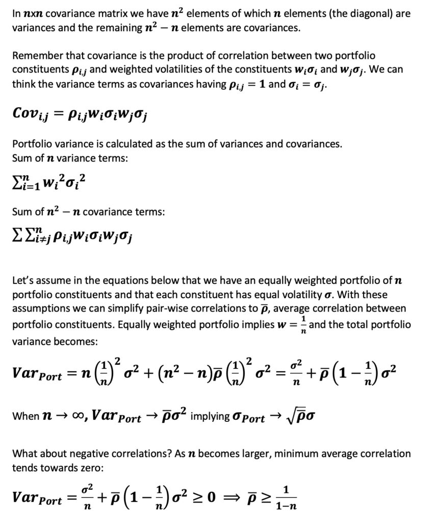
The effect of correlation on Sharpe ratio and its derivatives

To better understand diversification’s impact on a portfolio, we break down the covariance matrix and make simplifying assumptions. Our main assumptions include an equally weighted portfolio with equal constituent volatilities. With these assumptions, portfolio volatility approaches constituent volatility scaled by the square root of the average correlation as the number of constituents approaches infinity. In other words, as the number of constituents increases, the benefit of diversification is primarily determined by the average correlation.

Asserting a negative average correlation with more than a few constituents is a bold statement. Why is this the case? For instance, if a portfolio has 11 constituents with an average correlation of -0.1, the portfolio’s volatility would be zero, implying an arbitrage.

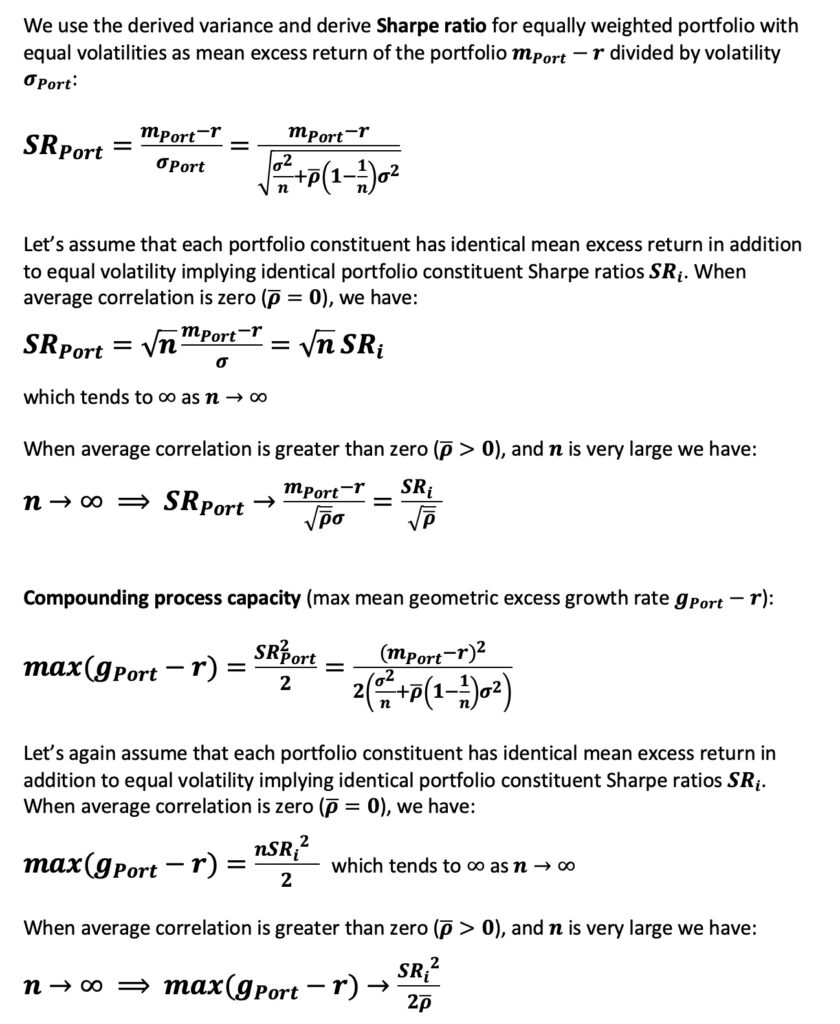
In addition to assuming an equally weighted portfolio and equal constituent volatilities, we also assume equal mean excess returns for the constituents, which implies equal Sharpe ratios. With these assumptions, we can express the portfolio’s Sharpe ratio and the maximum geometric mean excess return as functions of the constituent Sharpe ratio and the average correlation.

With zero average correlation, the portfolio’s Sharpe ratio is simply the constituent Sharpe ratio multiplied by the square root of the number of constituents. Similarly, the portfolio’s maximum mean excess growth rate is the constituent’s maximum mean excess growth rate multiplied by the number of constituents.

As the number of constituents approaches infinity, the portfolio Sharpe ratio approaches the constituent Sharpe ratio divided by the square root of the average correlation, while the portfolio’s maximum mean excess growth rate becomes the constituent’s maximum mean excess growth rate divided by the average correlation. Both the Sharpe ratio and the maximum mean excess growth rate become increasingly dominated by the average correlation as it rises from zero. Note that the growth rates derived from our equations are in a continuously compounded format.

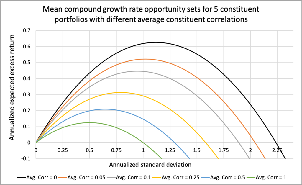
The figure below illustrates how the opportunity set for mean geometric excess returns—the increasing segment of the capital allocation parabola—expands significantly as the average correlation among portfolio constituents decreases. We have a portfolio consisting of five constituents, each with a Sharpe ratio of 0.5 and a volatility of 0.20.

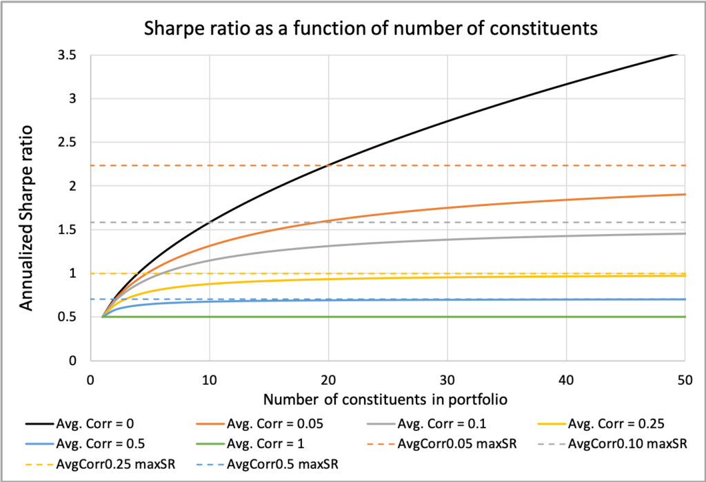
The next figure illustrates how the Sharpe ratio increases with the number of portfolio constituents. The extent of this increase and the potential for higher Sharpe ratios are heavily influenced by the average correlation among constituents. We observe that the Sharpe ratio quickly approaches its theoretical maximum, achievable at an infinite number of constituents, after only 10 constituents when the correlation is relatively high at 0.5. Conversely, even with 50 constituents, we are still far from reaching the maximum achievable Sharpe ratio when the average correlation is as low as 0.05. In the case of zero correlation, the portfolio Sharpe ratio continues to benefit from additional diversification, effectively approaching its maximum as the number of constituents increases indefinitely.

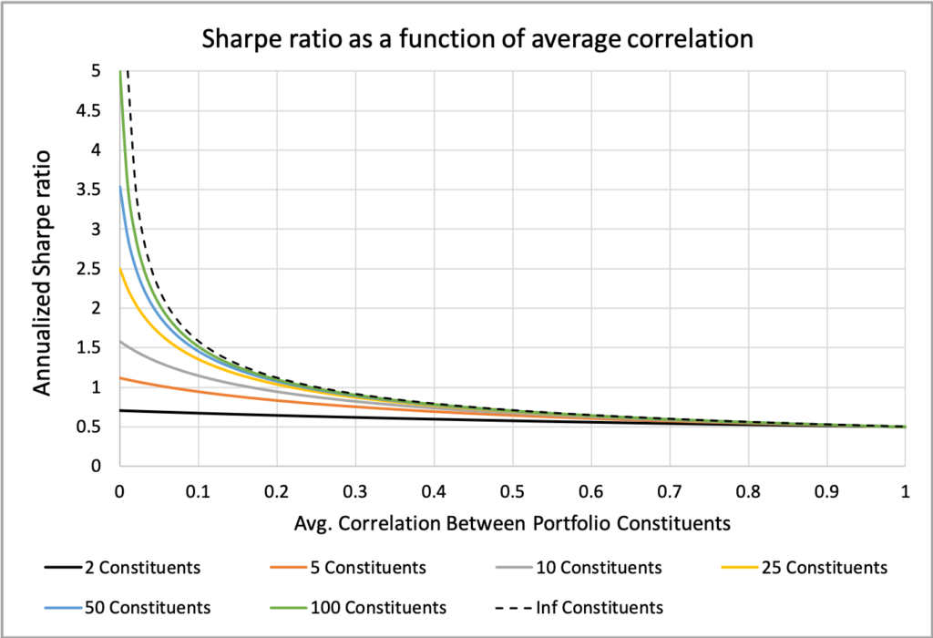
The figure below highlights that the effect of correlation on Sharpe ratio, or diversification benefit in general, is not linear. While we can enhance diversification by increasing the number of portfolio constituents, the increase in effectiveness really becomes apparent only at low correlation levels. For instance, a portfolio with 5 constituents at zero correlation performs as well as a portfolio with an infinite number of constituents with an average correlation of 0.2. Similarly, a portfolio with 2 constituents at zero correlation is equivalent to one with infinite constituents at an average correlation of 0.5.

The effect of correlation on the fraction of the full Kelly allocation

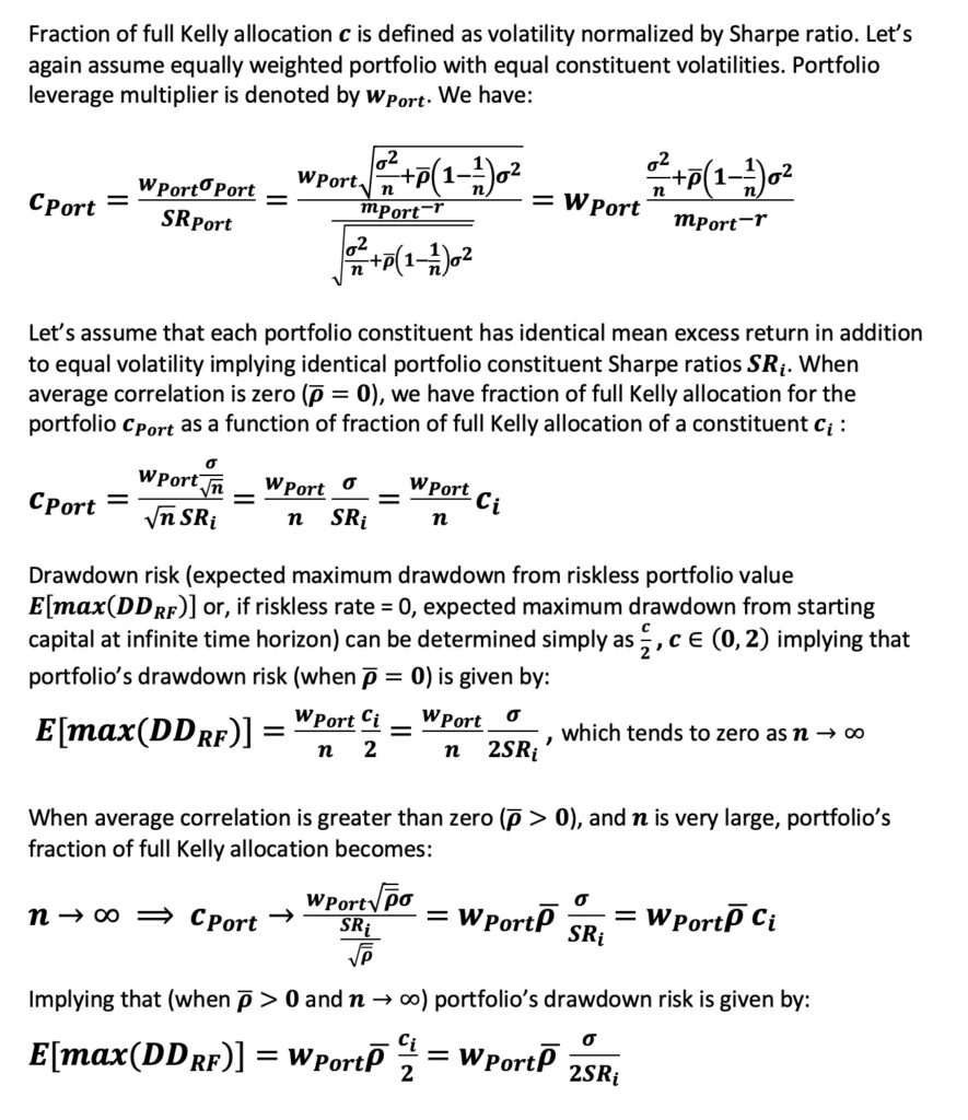
In my earlier article, Drawdown risk = portfolio volatility normalized by Sharpe ratio, we demonstrated that half of the fraction of the full Kelly allocation determines the expected drawdown from a riskless portfolio value (drawdown risk). We can interpret the fraction of full Kelly allocation, which is volatility normalized by Sharpe ratio, as a measure of portfolio risk instead of volatility.

In the case of uncorrelated constituents, assuming an equally weighted portfolio with constituents having equal volatility and mean excess return, the equations derived below show that the portfolio’s fraction of full Kelly allocation equals the constituent’s fraction of full Kelly allocation multiplied by the ratio of the leverage multiplier to the number of constituents. This means we can increase portfolio leverage in direct proportion to the number of additional uncorrelated constituents while keeping drawdown risk constant. Alternatively, we can maintain a constant portfolio leverage multiplier and reduce drawdown risk proportionally to the increase in the number of constituents.

When the average correlation is greater than zero and the number of constituents approaches infinity, the fraction of full Kelly allocation for an unleveraged portfolio approaches the constituent fraction of full Kelly allocation multiplied by the average correlation. This indicates that average correlation sets the limit for reducing drawdown risk or, alternatively, for leveraging potential if we aim to maintain constant drawdown risk.

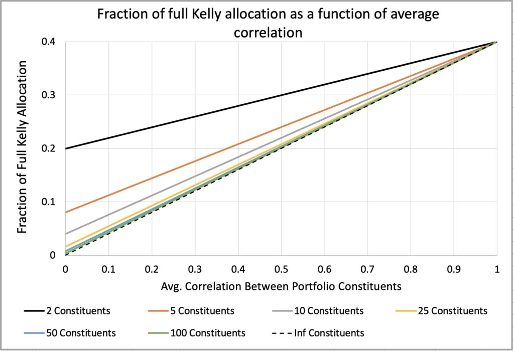
In the figure below, we maintain a constant portfolio leverage multiplier of one. We can observe that the fraction of full Kelly allocation decreases linearly as average correlation decreases. At zero correlation, the portfolio’s fraction of full Kelly allocation equals the constituent fraction of full Kelly allocation divided by the number of constituents.

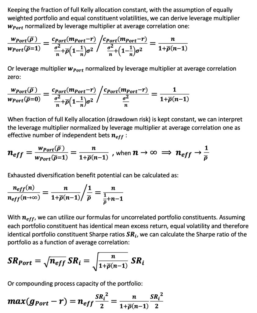
The equations below illustrate the metrics we can derive by keeping the portfolio’s fraction of full Kelly allocation (drawdown risk) constant while normalizing the leverage multiplier as a function of average correlation.

With our assumptions, we can normalize the portfolio’s leverage multiplier at a given average correlation by leverage multiplier at average correlation one. This yields the effective number of independent bets, a useful metric that quantifies the true diversification benefit as the number of portfolio constituents with zero cross-correlation. As mentioned earlier, two uncorrelated constituents are equivalent to an infinite number of constituents with an average correlation of 0.5. We can easily calculate this using the equation for effective number of independent bets.

Alternatively, we can normalize the portfolio’s leverage multiplier at a given average correlation by using the leverage multiplier at an average correlation of zero. This metric indicates how much we need to reduce our leverage if we wish to maintain constant drawdown risk while assuming zero correlation, but the actual correlation turns out to be higher than zero. The more constituents we have, the greater the required deleveraging in the event of a correlation spike.

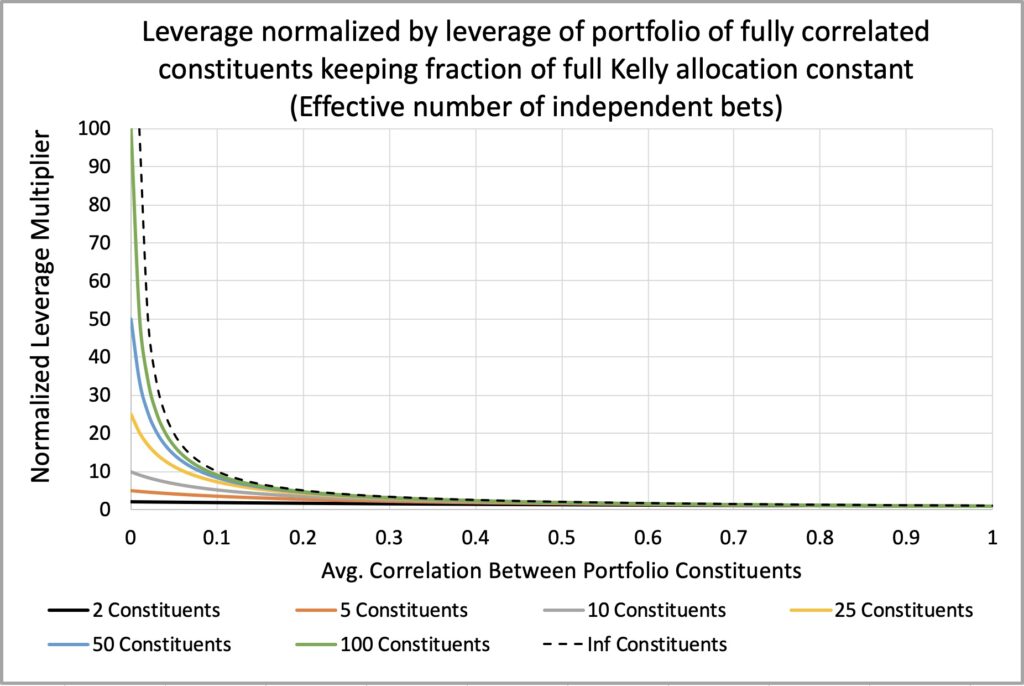
The figure below illustrates how the effective number of independent bets—essentially, the effective diversification benefit—significantly increases as we approach zero average correlation. At zero average correlation, the effective number of independent bets tends toward infinity as the number of portfolio constituents increases. In other words, the potential for diversification benefits is theoretically limitless when portfolio constituents are uncorrelated.

This figure can also be interpreted in terms of leveraging potential when the fraction of full Kelly allocation (drawdown risk) is kept constant. With 100 uncorrelated constituents, we can theoretically increase portfolio leverage by 100-fold compared to a single-constituent portfolio while maintaining a constant fraction of full Kelly allocation.

Leveraging a portfolio of uncorrelated constituents introduces correlation risk. As Corey Hoffstein puts it, “risk cannot be destroyed, only transformed.” When we assume zero (or any level lower than realized) average correlation while setting the portfolio leverage multiplier to achieve a desired risk level, we transform a significant portion of risk into correlation risk.

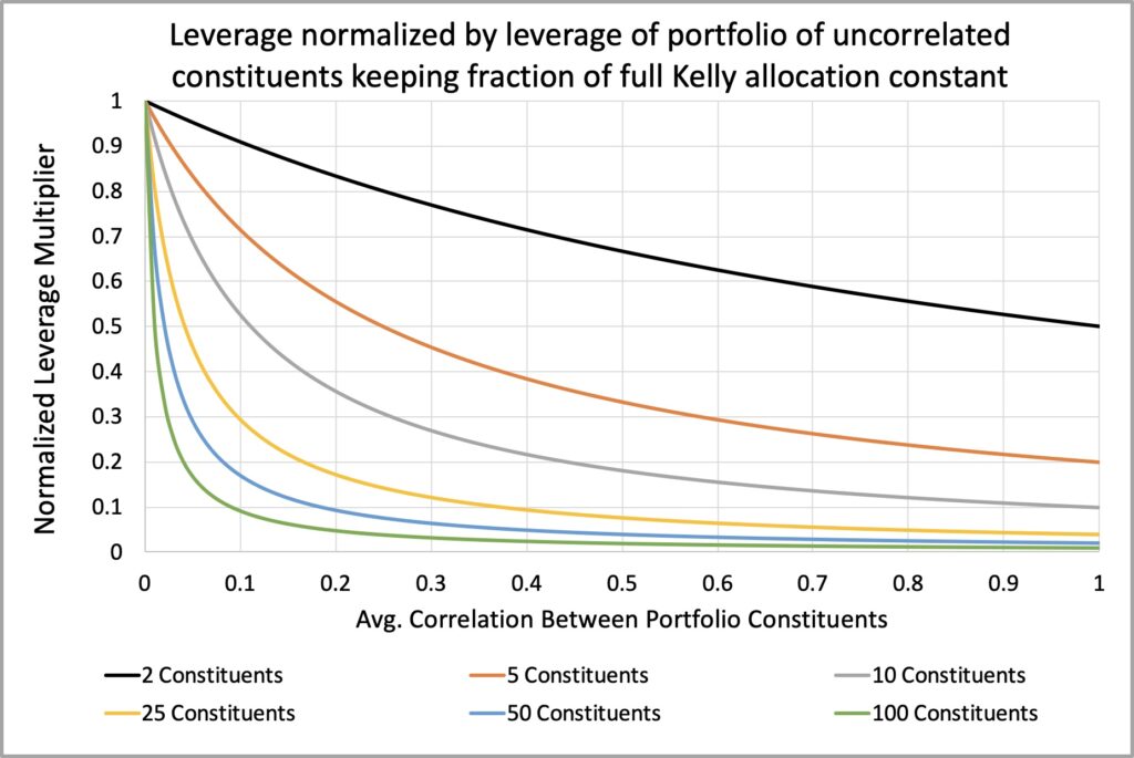
The next figure illustrates this correlation risk by plotting the required leverage multiplier divided by the original leverage multiplier (which is based on the zero correlation assumption). This is to show how much deleveraging is needed to maintain constant drawdown risk when the realized correlation is greater than zero.

Correlation risk increases significantly as the number of constituents in the portfolio increases. For instance, in a portfolio with 100 constituents, assuming zero correlation, the leverage multiplier must be reduced to about 9% of the original value when the average correlation reaches 0.1. If we fail to deleverage, the fraction of full Kelly allocation increases 10.9-fold (for example, a targeted 0.25 Kelly could surge to 2.725 Kelly).

In contrast, in the same scenario, a portfolio with just 5 constituents requires the leverage multiplier to be decreased to approximately 71% of the original value. Without deleveraging in this scenario, the fraction of full Kelly allocation rises 1.4-fold (for instance, a targeted 0.25 Kelly would increase to 0.35 Kelly).

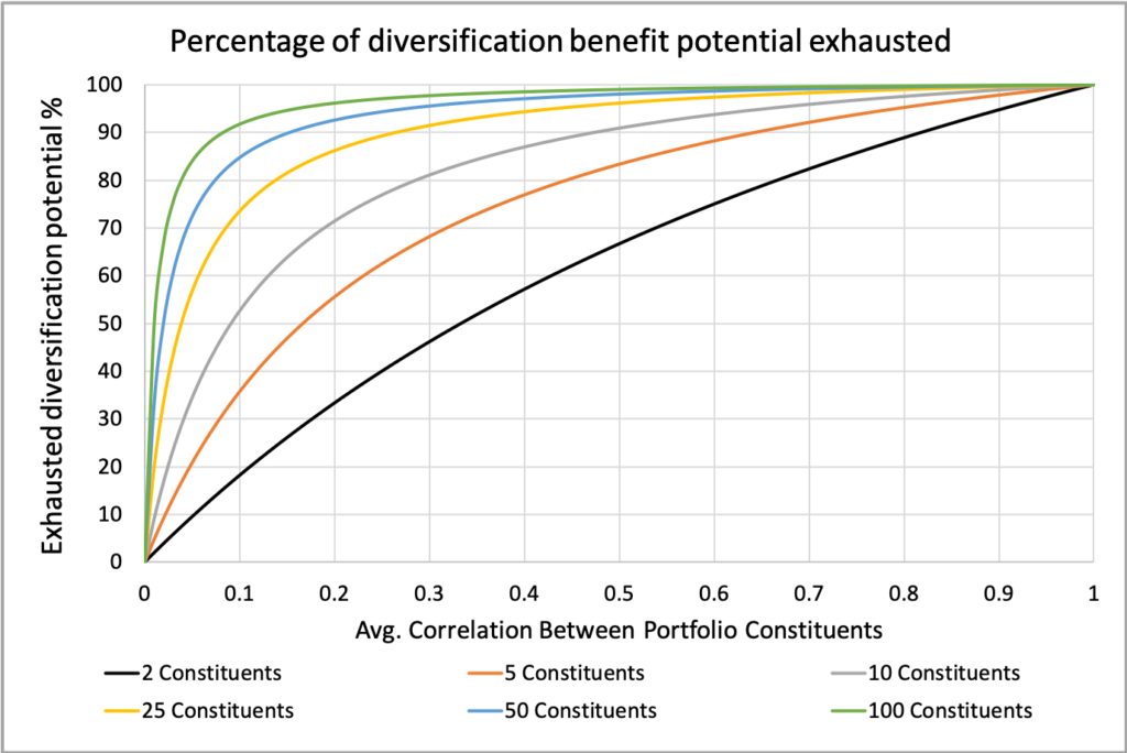
The figure below illustrates how much of the diversification benefit potential is exhausted as a function of average correlation. This metric compares the effective number of independent bets with n portfolio constituents to the effective number of independent bets with an infinite number of constituents.

It is evident that as the average correlation approaches zero, a greater number of portfolio constituents are required to fully exhaust the diversification benefit potential. For instance, with an average correlation of 0.5, approximately ten (specifically, nine) constituents have already utilized about 90% of the maximum diversification benefit. In contrast, when the average correlation is 0.1, nearly a hundred (specifically, eighty-one) constituents are necessary to exhaust 90% of the potential.

Simulating a portfolio of ten constituents

We have derived equations, and now we will put them to the test by executing a simple simulation. We simulate daily returns and create ten return series, each containing 12,600 samples (50 years × 252 trading days). The returns are drawn from a normal distribution. While the return series are initially uncorrelated, we introduce cross-correlation among the ten portfolio constituents and equalize their volatilities to 0.2 and their Sharpe ratios to 0.5, implying a mean excess return of 0.1.

Correlation among the constituents is established by exposing each return series to an eleventh return series, which has a mean excess return of 0.08, a volatility of 0.2, and a Sharpe ratio of 0.4. As a result, we have ten portfolio constituents with equal volatilities and Sharpe ratios but different exposures to the external factor. This external factor could represent, for example, a market or momentum factor. Alternatively, it could be a factor with zero or negative mean returns; however, in this example, we will focus on a factor with a positive mean. Let’s say it is an exposure to the market.

The figure below displays the correlation matrix of our equally weighted, daily rebalanced portfolio. The average cross-correlation among the portfolio constituents is 0.24. The resulting portfolio has a mean excess return of 0.1, a volatility of 0.112, and a Sharpe ratio of 0.89. Additionally, our portfolio has a market beta of 0.5.

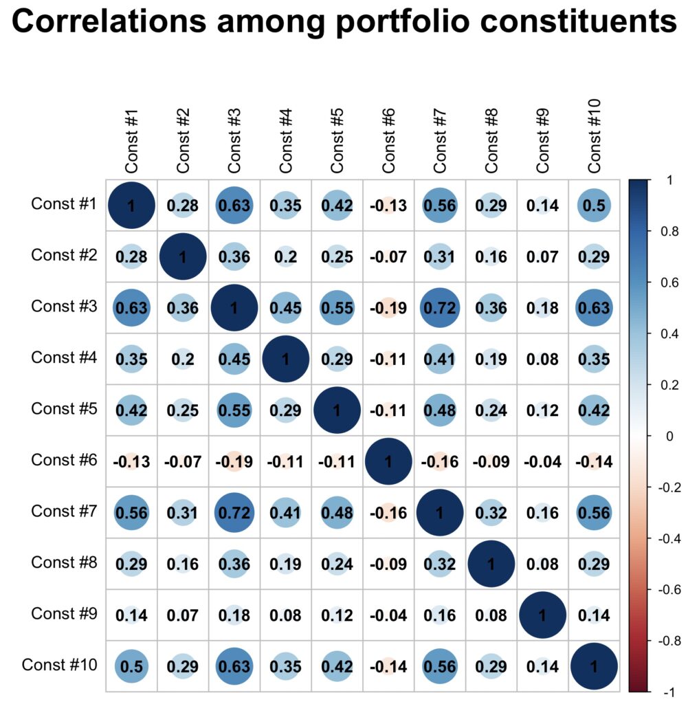
We create three portfolios. The first is the original portfolio described above. The second is a fully hedged portfolio (hedge ratio = 1), in which we have completely removed the market beta of 0.5 through hedging. In the fully hedged portfolio, both the market beta and the average cross-correlation between the constituents are zero. The third portfolio is a Sharpe optimally hedged portfolio.

Fully hedged portfolio has a mean excess return of 0.06, a volatility of 0.0512 and a Sharpe ratio of 1.17. We can utilize the formula we derived and calculate the Sharpe optimal hedge ratio as 1 – (0.0512*0.4)/(0.5*0.2*1.17) = 0.825. This means we don’t hedge 100%, but 82.5% of the market beta. This is achieved by shorting 0.825*0.5 = 0.4125 times the market, which leaves our Sharpe optimally hedged portfolio with 0.5 – 0.4125 = 0.0875 market beta, thereby maximizing the Sharpe ratio of the portfolio.

The mean excess return of the Sharpe optimally hedged portfolio is 0.067, with a volatility of 0.054 and a Sharpe ratio of 1.24. Notice that, due to hedging a positive mean factor, the mean excess return of both hedged portfolios is substantially lower than that of the original portfolio. Intuitively, this may not sound like a smart move, but the key point is that the Sharpe ratio—and therefore the compounding process capacity—is higher with hedging.

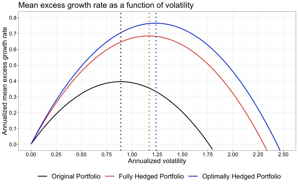
The figure below shows the capital allocation parabolas, which represent the mean geometric excess return as a function of volatility for the three portfolios. This figure illustrates the power of low correlation and high Sharpe ratios. The two portfolios with the highest maximum returns (and, consequently, the highest compounding process capacities) have substantially higher Sharpe ratios compared to the original portfolio. Therefore, when leverage is applied, we have an extended opportunity set for selecting our preferred risk and reward, and the risk-adjusted mean growth rate is clearly superior to that of the lower Sharpe portfolio.

The optimally hedged portfolio has a higher Sharpe ratio than the fully hedged portfolio. However, it is not straightforward to declare the highest Sharpe portfolio as the best option. We must distinguish between a building block and a building. If we are constructing a portfolio (the building), then the optimally hedged portfolio, with its higher Sharpe ratio, can be considered superior to the fully hedged portfolio.

On the other hand, if we are creating an asset (a building block) to be added to a larger portfolio, the fully hedged portfolio may be more advantageous. This is because factor returns (especially the market factor) are ubiquitous, and your larger portfolio probably already has exposure to these factors or can gain such exposure more efficiently elsewhere.

If your building block is contaminated with factor exposures, it is essential to consider your current exposures and optimize the new building as a whole when integrating the new building block into your existing portfolio. A pure alpha portfolio (a portfolio with no factor exposures) can be regarded as an optimal plug-and-play building block, as it is orthogonal to any other constituents you may have in your existing portfolio.

We can use the formula for the effective number of independent bets for our original portfolio, which gives us 10/(1 + 0.24*(10 – 1)) = 3.165. From this, we can calculate the Sharpe ratio: sqrt(3.165)*0.5 = 0.89. Next, we can compute the compounding process capacity (maximum mean excess growth rate) as (3.165*0.5^2)/2 = 0.396, which aligns with our simulation. The maximum mean excess growth rates for the fully hedged and optimally hedged portfolios can be calculated based on their Sharpe ratios, yielding 1.17^2/2 = 0.684 and 1.24^2/2 = 0.769, which also agree with our simulation results.

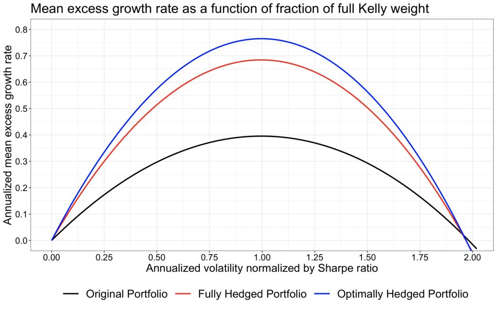
We can interpret the fraction of full Kelly allocation—technically, volatility normalized by the Sharpe ratio—as a risk measure for our portfolio. This perspective is particularly justified if we consider drawdown to be a more relevant risk measure than volatility.

In the next figure, we plot the capital allocation parabolas as a function of volatility normalized by the Sharpe ratio. Theoretically, we expect the parabolas to be perfectly symmetrical and to reach zero mean excess growth rate exactly when the fraction of full Kelly allocation equals 2. However, we observe that the parabolas dip into negative territory slightly before this point. This discrepancy arises because we rebalance daily, whereas the theoretical model assumes continuous rebalancing. Nevertheless, the difference is barely noticeable.

Using the fraction of full Kelly allocation as a risk measure, particularly when considering the relevant rising half of the parabola, the difference in risk-adjusted returns between portfolios is even more pronounced than when volatility is used as a risk measure. This indicates that if we regard drawdown as our primary risk measure instead of volatility, the significance of the Sharpe ratio increases even further from its already esteemed position in a framework where volatility is considered synonymous with risk.

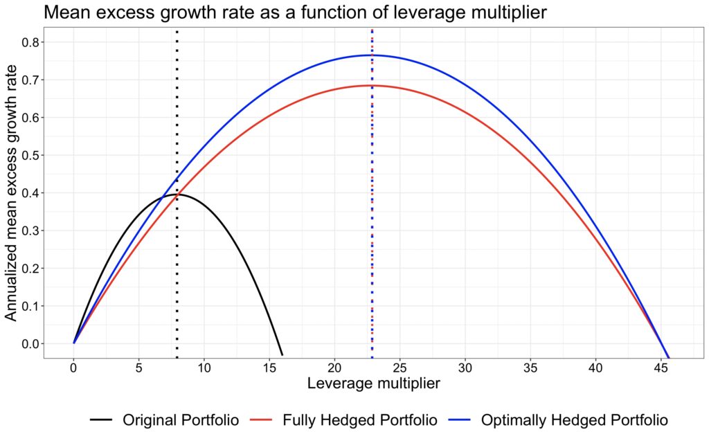
Finally, we plot the parabolas as a function of the leverage multiplier. Here, we can clearly see that a high Sharpe ratio requires leverage to unlock the benefits of diversification and achieve a sufficiently high mean growth rate. Our original portfolio has the highest unleveraged mean excess growth rate and outperforms if the investor is unwilling or unable to use leverage and requires relatively high returns. However, the cost of utilizing a low Sharpe portfolio carries a high risk, manifested in both volatility and drawdowns. Of course, in real life, the cost of borrowing would lower the parabolas. In our simulations, we assume lending and borrowing occur at the riskless rate.

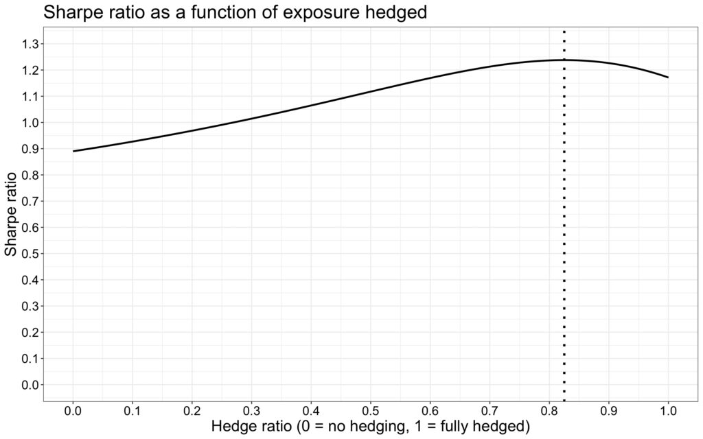
Our last figure illustrates how the Sharpe ratio of the portfolio evolves as a function of the hedge ratio (the ratio of hedged factor exposure to the full hedge). We can see that the maximum Sharpe ratio is achieved when 82.5% of the full hedge is utilized. However, the key takeaway from the figure is that the Sharpe ratio is not very sensitive to getting the hedge ratio exactly right. Essentially, it suggests that you should hedge, but not necessarily to the full extent if your goal is to increase your Sharpe ratio. Conversely, if you are aiming for a pure alpha portfolio—essentially a building block rather than a building—you should theoretically hedge fully.

Conclusions

The capital allocation parabola and its maximum, compounding process capacity, define the opportunity set available to investors who care about geometric mean returns. These concepts can be extended beyond stock diversification to enhance our understanding of the power of diversification across uncorrelated portfolio constituents.

The maximum mean geometric excess return of a portfolio composed of uncorrelated constituents—referred to as compounding process capacity—equals one half of the sum of the squared constituent Sharpe ratios. Each constituent is optimally weighted by its full Kelly weight, which is calculated as the Sharpe ratio divided by its volatility. The full Kelly weight of the portfolio is simply the sum of the full Kelly weights of its constituents.

To determine the variance ratio that maximizes the Sharpe ratio of the portfolio, we can utilize the ratio of the squared Sharpe ratio of the factor portfolio to the sum of the squared Sharpe ratios of both the factor portfolio and the fully hedged portfolio.

For an equally weighted portfolio of constituents with equal volatility and Sharpe ratio, the Sharpe ratio of the portfolio is simply the constituent Sharpe ratio multiplied by the square root of the effective number of independent bets. The maximum mean excess geometric return of the portfolio is equal to one half of the squared constituent Sharpe ratio multiplied by the effective number of independent bets. Notably, the effective number of independent bets equals the number of constituents when the average correlation among them is zero.

When the average correlation among constituents is greater than zero, the Sharpe ratio of the portfolio approaches the constituent Sharpe ratio divided by the square root of the average correlation as the number of constituents increases towards infinity. Consequently, the maximum mean excess geometric return of the portfolio approaches one half of the square of the constituent Sharpe ratio divided by the average correlation. In general, the diversification benefit is more constrained by average correlation than by the number of constituents.

An infinite number of uncorrelated portfolio constituents theoretically results in an infinite Sharpe ratio, leveraging potential, and compounding process capacity. Thus, having a substantial number of uncorrelated constituents combined with meaningful leverage is an attractive goal. However, monetizing the assumption of zero or very low correlation among numerous constituents through the use of leverage exposes the portfolio to considerable correlation risk. Even a slight increase in average correlation may necessitate rapid and substantial deleveraging to maintain tolerable drawdown risk.

Hedging factor exposures results in a pure alpha portfolio, which, assuming a positive alpha, serves as a perfect orthogonal building block for a portfolio. Sharpe optimal hedging may require a partial hedge, which can enhance the overall portfolio, leading to a higher Sharpe ratio. The benefits of hedging largely depend on the effective utilization of leverage to unlock the benefits of diversification. In many instances, diversification without adequate leverage results in a low-risk, low-reward scenario. Conversely, diversification combined with sufficient leverage can create a desirable balance of risk (often largely in the form of correlation risk) and meaningful rewards.

References

[1] Kenneth French data library

[2] Wikipedia: Maximum-ratio combining

[3] Thorp, E. O. (2006). The Kelly criterion in blackjack, sports betting and the stock market

[4] Paleologo, G. A. (2021). Advanced Portfolio Management: A Quant’s Guide for Fundamental Investors

Article by Markku Kurtti