
We will show that the single best metric predicting drawdown risk is portfolio volatility normalized (divided) by Sharpe ratio i.e. fraction of full Kelly allocation.
We first derive the formulas for drawdown probabilities and expected drawdowns, then verify the formulas by simulations and finally demonstrate with empirical data.
With the exception of the effect of empirical return time series autocorrelation, empirical drawdown risk is shown to be accurately predicted by theoretical formulas and to match (i.i.d.) simulated drawdown risk.
Is risk measured by volatility or by volatility normalized by Sharpe ratio?
Conventional finance theory defines risk as volatility – the standard deviation of returns. Volatility conveys the uncertainty related to expected return.
Practitioners, on the other hand, often measure and care more about drawdowns.
One way to compare these two risk measures is thought experiment with imaginary portfolios A and B.
Portfolio A: annualized mean excess return 0.06, volatility 0.15, Sharpe ratio 0.4, volatility normalized by Sharpe ratio i.e. fraction of full Kelly allocation c = 0.15/0.4 = 0.375. Portfolio B: annualized mean excess return 0.40, volatility 0.20, Sharpe ratio 2.0, volatility normalized by Sharpe ratio i.e. fraction of full Kelly allocation c = 0.2/2.0 = 0.1.
Conventional finance theory says that portfolio B is 0.2/0.15 = 1.33 times riskier than portfolio A, because it has higher volatility. But is it really riskier?
Portfolio B has phenomenally high expected return, but slightly higher volatility than portfolio A. Slightly higher volatility means slightly higher spread around the expected excess return. But with such very high expected excess return, does it really matter if your annual return is sometimes one standard deviation lower than the expectation but still at very high level: 0.40 – 0.20 = 0.20. Or if we have a really bad year and are down by two standard deviations at excess return 0.4 – 2×0.2 = 0. Compare that to portfolio A being down two standard deviations at excess return level 0.06 – 2×0.15 = -0.24.
On the other hand, when we consider portfolio volatility normalized by Sharpe ratio i.e. fraction of full Kelly allocation c, we notice that portfolio A is vastly riskier. Portfolio A is 0.375/0.1 = 3.75 times riskier than portfolio B. As we will show later in this post, portfolio A has 3.75 times higher drawdown risk compared to portfolio B.
As a summary: Based on volatility, portfolio B is 1.33 times riskier compared to portfolio A. Based on portfolio volatility normalized by Sharpe ratio, portfolio A is 3.75 times riskier than portfolio B.
The point is that drawdown (portfolio volatility normalized by Sharpe ratio) as a risk metric incorporates not only volatility but also expected excess return. The higher the expected excess return, the higher the Sharpe ratio and the lower the expected drawdown.
There are good reasons why so many practitioners prefer drawdown (indirectly prefer volatility normalized by Sharpe ratio) over volatility when they assess risk.
Drawdown math
To derive the needed equations, we only need to read and apply Ed Thorp’s classic on the Kelly criterion [1]. For more background on the Kelly criterion, you may check my earlier post: The Kelly criterion, capital market parabola & the almighty Sharpe ratio.
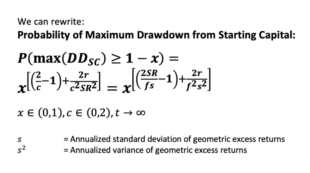
The equation below determines the chance of ever falling to portfolio value lower or equal to x times the starting capital. One way to assess drawdown is to consider maximum drawdown from starting capital, which is part of the equation.
Notice that the fraction of fully Kelly allocation c is determined by portfolio volatility fs normalized (divided) by Sharpe ratio SR. Portfolio volatility is equal to unlevered portfolio volatility s multiplied by leverage multiplier f (investment fraction).
Fraction of full Kelly allocation c, portfolio volatility normalized by Sharpe ratio, is either the dominant or the determining term in all of the drawdown formulas we derive.
The equations assume continuously compounded returns to be used when calculating the inputs.

We can express the equation as a probability of maximum drawdown from starting capital:
The best overall definition for drawdown risk is expected drawdown (expected drawdown depth). We show below how to derive expected maximum drawdown from starting capital.
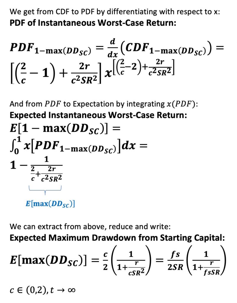
Expected maximum drawdown from starting capital is dominated by term c, fraction of full Kelly allocation. Risk-free return provides some cushion.
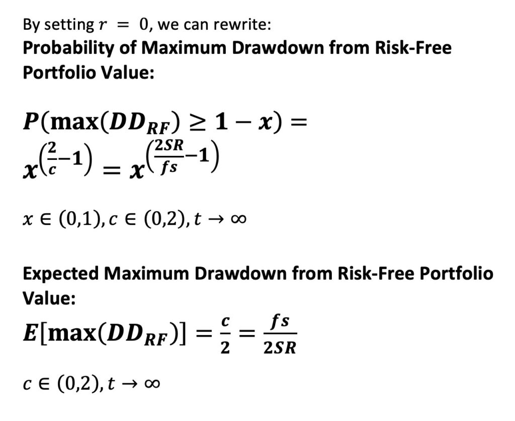
Below we set the risk-free return to zero. This can be interpreted as expected maximum drawdown from starting capital in zero interest rate environment, but – more interestingly – we can interpret it as setting the risk-free rate as a reference level. Having risk-free rate as a reference level allows us to interpret the equations as maximum drawdown from risk-free portfolio value. Instead of calculating the drawdown from starting capital (at time = 0), we now calculate the drawdown from current risk-free portfolio value (the current value of compound risk-free rate).
Deviation from risk-free portfolio exposes investor to risk: drawdown from risk-free portfolio value. Maximum drawdown from risk-free portfolio value is very useful risk metric as it takes opportunity cost (risk-free investment) into account. Having a drawdown from risk-free portfolio value indicates you would have been better off by not taking any risk. Maximum drawdown from risk-free portfolio value therefore captures the maximum regret of taking risk.
Expected maximum drawdown from risk-free portfolio value – the expected maximum regret of taking risk – is beautifully captured by c/2, one half of fraction of full Kelly allocation (one half of portfolio volatility normalized by Sharpe ratio).
Notice that the equation of probability of maximum drawdown from risk-free portfolio value is essentially the same as Thorp’s eq. 7.13 [1].
Simulations & empirical results
All simulations and empirical tests use daily data between Jul-1926 and Jun-2021 from Kenneth French data library [2]. Risk-free return is monthly T-bill. Using daily data is essential when assessing drawdowns as monthly data would downplay drawdown depth by smoothing the data. Our theoretical equations assume returns measured at infinitely short intervals, but daily is close enough.
Our equations assume infinite time horizons. We will simulate different time horizons to test how the theoretical predictions work on different time horizons.
In the simulations we draw daily Laplace (i.i.d.) distributed excess returns and create parallel return histories for each time horizon. We use fat-tailed Laplace distribution, which shape is closely matched with empirical daily return distribution shape. However, as our simulation data is i.i.d., central limit theorem works very effectively and it doesn’t really matter in the long-term whether we use normally distributed or Laplace distributed daily data.
We have shown in an earlier post The Kelly criterion, capital market parabola & the almighty Sharpe ratio that the interesting range of the fraction of full Kelly fraction c is from zero to one. This is because expected growth rate of the portfolio will start to decrease when c > 1. We therefore are mostly interested in drawdowns in the range 0 < c ≤ 1.
Maximum drawdown from risk-free portfolio value
In the simulations, we use empirical parameters and create 20000 parallel i.i.d. return histories for each time horizon except for 5000-year horizon, for which 10000 histories are created. We use excess returns corresponding to ”Mkt-RF” in the empirical Kenneth French data. Annualized empirical daily mean arithmetic excess return is 8.1%, volatility 17.5% and Sharpe ratio 0.46.
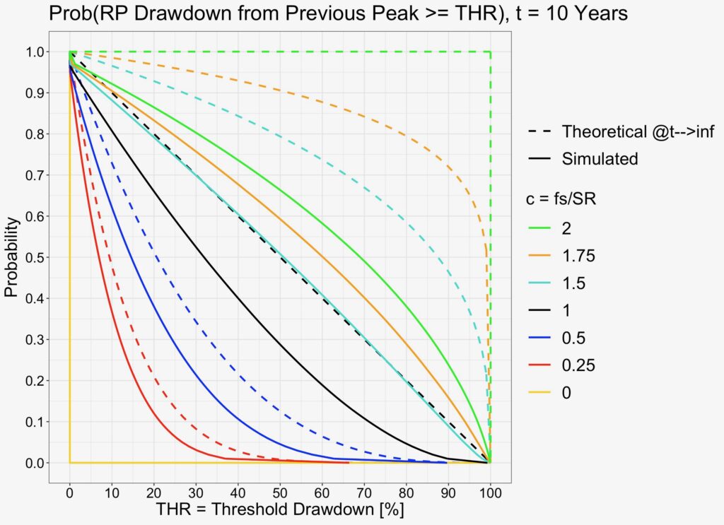
Already with 10-year time horizon, we can see that – in the relevant range 0 < c ≤ 1 – simulated maximum drawdown probabilities are reasonably close to theoretical predictions.

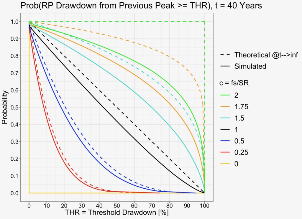
At 40-year horizon, relevant fractional Kelly values have practically converged to their theoretical prediction.

At 100-year horizon, c values up to 1.5 have converged.

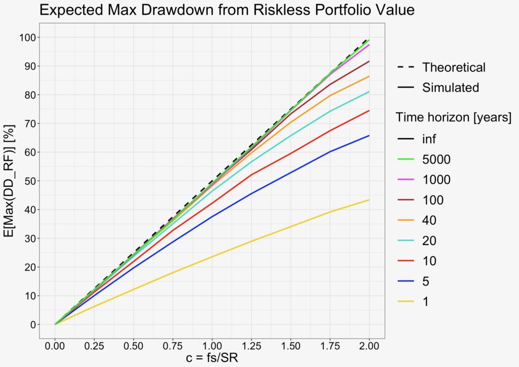
And finally (in the figure below), using 5000-year horizon, we verify that the equation works in the whole range 0 < c < 2.
What this figure tells us is that you are sure to hit close to 100% maximum drawdown and to meet you uncle point in the very long-term when you approach c = 2 i.e. when your portfolio volatility approaches two times your Sharpe ratio. Your expected excess growth rate turns negative only after c > 2. This means that negative expected growth rate is not needed to ruin your portfolio as expected maximum drawdown approaching 100% will ensure your ruin. It is not the growth rate but the drawdowns that will kill excessive risk takers.
Also, at full Kelly allocation (c = 1), linearly increasing cumulative maximum drawdown probability implies that the probability density function (PDF) of the maximum drawdown is flat (continuous uniform distribution). This means that any maximum drawdown from risk-free portfolio value is equally likely. A drawdown of 0% to 1% and drawdown of 99% to 100% are equally likely. At full Kelly, having an uncle point at 40% drawdown, you have a 60% probability of ruin in the long-term. Even if you can tolerate up to 75% drawdown, your probability of ruin is still 25%. You can imagine the amount of uncle points met at full Kelly allocation. And in reality, the parameters determining full Kelly allocation are uncertain estimates, making it even more risky to target full Kelly.
Lowering risky asset allocation quickly decreases your maximum drawdown probability. At full Kelly (c = 1) your probability of maximum drawdown of 50% or more is 50%. At half Kelly (c = 1/2), the probability drops to 12.5% and at quarter Kelly (c = 1/4) to less than 0.8%.

Next, we simulate expected maximum drawdown from risk-free portfolio value. The equation is simply half of fraction of full Kelly allocation – half of portfolio volatility normalized by Sharpe ratio.
We can see from the figure below how longer time horizon helps to converge the curve towards the predicted linear function. 20 to 40 years is enough to achieve convergence in the relevant range 0 < c ≤ 1.
Clearly, the equations work in i.i.d. simulation. But how about the empirical data?
Long-term empirical tests are tricky as we have so little data. One 95-year period really isn’t much compared to e.g. 10000 parallel 5000-year periods (= 50 000 000 years) we just simulated.
With the limited empirical data that we have, we can try rolling windows by rolling the window with one day steps. We test 1-, 5- and 10-year windows over the 95-year empirical data, which gives us 95, 19 and 9.5 independent periods.
In the figure below, we plot the theoretical expectation (at infinite time horizon) and i.i.d. simulated curves for reference. Empirical result is relatively close to simulated curves, but the shape of the curves clearly is curvier.
Empirical maximum drawdown from risk-free portfolio value in the relevant range is worse (greater) than i.i.d. simulated reference. This means (excluding the curvier shape) that the maximum drawdown from risk-free portfolio is relatively accurately predicted by the theoretical equation (which assumes infinite horizon) already at 5- to 10-year empirical horizons in the range of 0 < c ≤ 1.
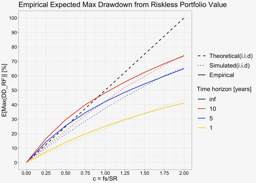
What is the difference between the i.i.d. simulations and the empirical data? It is the return time series autocorrelation (e.g. time series momentum) which is present in the empirical data.
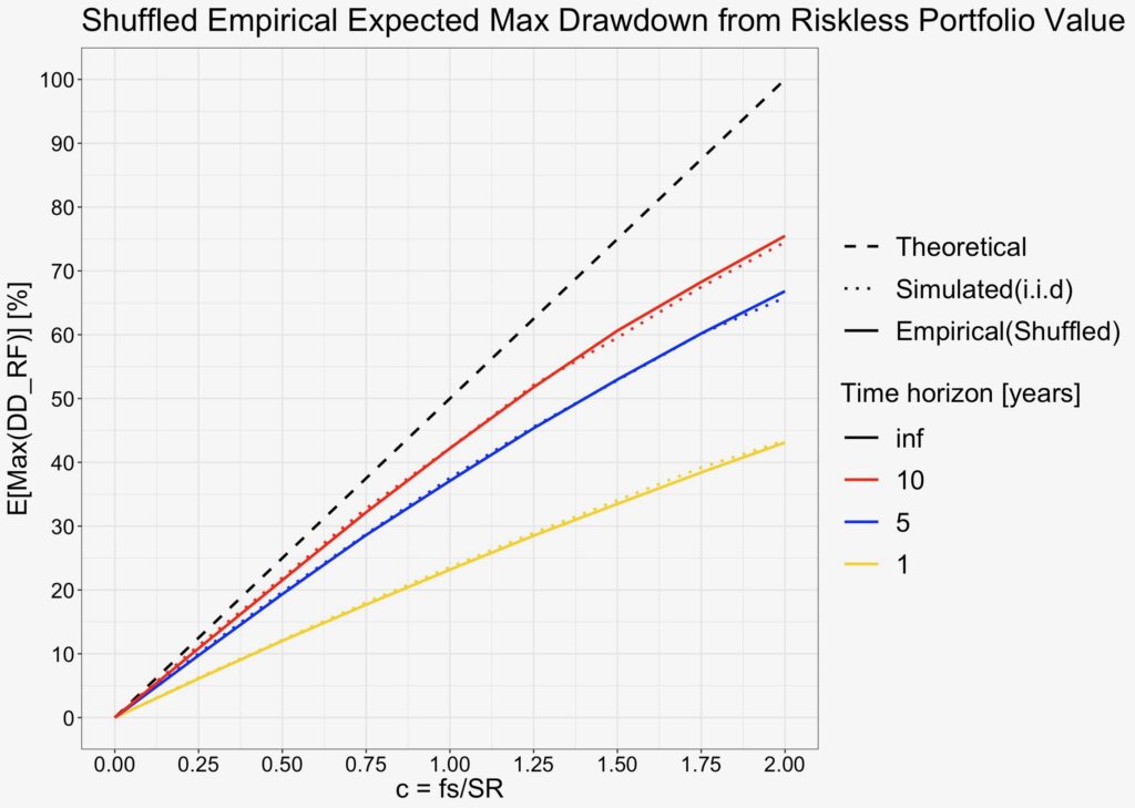
An easy way to get rid of autocorrelation is to reshuffle the daily return data. We randomly shuffled the data, calculated the maximum drawdown from risk-free portfolio value 500 times for each test point and calculated an average over the 500 results for each test point. As can be seen from the figure below, the average of shuffled data closely follows i.i.d. simulated results. This tells us that it is the autocorrelation that causes the curvier shape.
Maximum drawdown from starting capital
We can simulate also the maximum drawdown from starting capital. Now the risk-free return is included and provides some cushion against drawdowns. Drawdown now needs to first consume the gains compounded by risk premium and then consume the gains compounded by the risk-free rate to reach below the starting capital level. We use empirical parameters in the simulation. Empirical annualized mean risk-free rate is 3.2%.
In the simulations, we create 20000 parallel i.i.d. return histories for 10- and 40-year horizons and 10000 histories for 100- and 1000-year horizons.
We can see from the figure below that simulated values converge to their theoretical predictions at 1000-year horizon. Also, when comparing to maximum drawdown from risk-free portfolio value, we can see that risk-free rate provides small cushion and drawdowns are slightly less severe. But in the big picture, the figure is the same what we saw in the case of maximum drawdown from risk-free portfolio value.

The expected maximum drawdown from starting capital is not exactly a straight line anymore, but slightly curved. Also, thanks to risk-free return component, expected maximum drawdown no longer approaches 100% (more like 93% now) when c approaches 2.

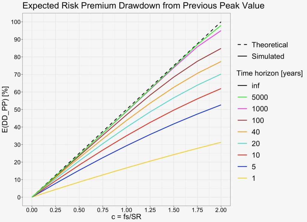
Risk premium drawdown from previous peak value
It turns out in the simulations, that it is not only the maximum drawdown from risk-free portfolio value or from starting capital which obey the derived equations.
We find that the probability of risk premium drawdown from previous peak value (measured over all time instants) is determined by the same formula as the probability of maximum drawdown from risk-free portfolio value. And the same goes for the expected risk premium drawdown from previous peak value, which is determined by the same formula as the expected maximum drawdown from risk-free portfolio value.
Also, we find that probability and expected value of portfolio drawdown from previous peak value (measured over all time instants) is determined by the same formulas as the probability and expected value of maximum drawdown from starting capital.
In the simulations, we create 5 000, 2 000, 1000 and 1000 parallel i.i.d. return histories for 10-, 40-, 100- and 5000-year horizons, respectively. We don’t need as much data in simulations compared to simulations for maximum drawdown from risk-free portfolio value, because now, instead of measuring one maximum drawdown per return history, we measure the drawdown for each day.
We can see in the probability figures below that simulated curves again converge towards their theoretical prediction, but more slowly compare to maximum drawdown from risk-free portfolio value simulations.
Probabilities are now calculated for an arbitrary time instant between portfolio formation and the time horizon length (which in the theoretical case is infinity).


We can see from the figure below that it now takes about 100 years for the expectation to achieve convergence in the relevant range 0 < c ≤ 1.
Expected risk premium drawdown from previous peak value can be interpreted as the average regret (averaged over all time instants) of not selling at the previous risk premium peak value.
We again test with empirical data and find that empirical expected risk premium drawdowns from previous peak values are slightly lower compared to i.i.d. simulated values.

We again re-shuffle the daily excess returns and find that the average of shuffled results matches with i.i.d. simulations. Empirical time series autocorrelation makes the risk premium drawdown from previous peak slightly milder than i.i.d. simulations suggest.

Portfolio drawdown from previous peak value
When investors hear “drawdown” they usually think portfolio drawdown from previous peak value. Portfolio return includes both risk premium and risk-free rate, and risk-free rate therefore – similarly as in the case of maximum drawdown from starting capital – provides some cushion against drawdowns.
Simulations below verify that the equations work. We can see that drawdowns are not quite as severe as in the case when we don’t have cushion from risk-free rate (maximum drawdown from risk-free portfolio value & risk premium drawdown from previous peak value), but in the big picture they all look the same and are dominated by the portfolio volatility normalized by Sharpe ratio – the fraction of full Kelly allocation.
Expected portfolio drawdown from previous peak value can be interpreted as the average regret (averaged over all time instants) of not selling at the previous portfolio peak value.


Conclusions & Implications
Apart from empirical return time series autocorrelation, both drawdown probabilities and expectations are either fully determined or dominated (when other parameters affect drawdown) by portfolio volatility normalized by Sharpe ratio.
With the exception of empirical return time series autocorrelation, fraction of full Kelly allocation (portfolio volatility normalized by Sharpe ratio) divided by two determines expected maximum drawdown from risk-free portfolio value and risk premium drawdown from previous peak value. The same metric dominates expected maximum drawdown from starting capital and expected portfolio drawdown from previous peak value, which both are gently tempered with the help of risk-free return.
Empirical autocorrelation makes expected maximum drawdown from risk-free portfolio value more severe than expected based on i.i.d. based simulations. On the other hand, empirical autocorrelation makes expected risk premium drawdown from previous peak value less severe compared to i.i.d. simulations. Autocorrelation seems to make drawdown extremes (maximum drawdowns) more severe while typical drawdowns are tempered. On balance, we can consider autocorrelation as increasing the drawdown risk as it is the extreme drawdowns which tend to lead to ruin.
Approaching fraction of full Kelly allocation c = 2, i.e. portfolio volatility normalized by Sharpe ratio at value two, leads to 100% expected maximum drawdown from risk-free portfolio value (and to or close to 100% expected drawdown with all the metrics we tested) marking a certain portfolio ruin in the long-term. At this point expected portfolio growth rate is still positive implying that, by expectation, ruin is not caused by negative growth rate but drawdown.
For practitioners who perceive drawdowns as risk, portfolio risk is not measured by portfolio volatility, but by portfolio volatility normalized by Sharpe ratio.
References
[1] Thorp, E. O. (2006). The Kelly criterion in blackjack, sports betting and the stock market
[2] Kenneth French. ‘Fama/French 3 Factors [Daily]’ Kenneth French data library
Article by Markku Kurtti