The Kelly criterion, capital market parabola & the almighty Sharpe ratio

Expected return is at the center of financial analysis. But when you hear expected return, you can’t be sure if it is geometric expectation (time average) or arithmetic expectation (ensemble average). Almost without exception, investors mentioning expected return mean geometric expected return. One reason is that realized historical returns are geometric. But more importantly, long-term investors want to grow their wealth over time through compounding and compounded returns are geometric returns. See more about time and ensemble averages and the so-called ergodicity problem from Peters [1].

Contrary to practitioners, expected return in the terminology of conventional finance theory means expected arithmetic return (ensemble average). In the return time series, expected arithmetic return describes the average of single period returns (e.g. an average of an ensemble of daily returns).

In practice, after an individual investor has reached his limits of portfolio diversification – be it because of exhausting available assets, preference for concentrated portfolio or any other reason – the investor only has one available dimension (path) with his portfolio and this dimension is through time. Arithmetic (ensemble) average describes the expectation over an ensemble of such paths, but long-term investors only have one life to live and invest. Therefore – after reaching the limits of diversification – long-term investors should use geometric expectation (time average) when assessing the expectation of their long-term portfolio returns.

We will see how the difference between the two types of expected returns makes a big difference when deciding how much of your portfolio to allocate to risky assets when investing over time. The Kelly criterion helps us to understand the world of geometric returns and particularly the effect of risky asset allocation and leverage. We will see how linear transforms to parabolic – including the transformation of capital market line into capital market parabola – as we move from the world of arithmetic to the world of geometric expectation.

The somewhat intangible meaning of Sharpe ratio becomes more tangible as we move our analysis into the world of time averages. We will find how the importance of Sharpe ratio is even more pronounced in the world of time averages where it not only determines the efficient portfolio, but determines and limits the whole risk & reward opportunity set available to investor who cares about risk adjusted or the maximum geometric expected return.

Finally, we compare the geometric expected excess growth rates predicted by theory to those obtained with empirical data. We find that – despite the well documented fat tailedness and autocorrelation of empirical returns – theoretical fractional Kelly criterion accurately predicts empirical outcomes as long as we rebalance our risky asset allocation back to target with a high enough frequency. 

The fractional Kelly criterion

Claude Shannon, one of the greatest scientists of the 20th century, invented information theory (and published it in 1948 [2]), which determined a mathematical upper bound – information channel capacity, the Shannon limit – for average error free information exchange rate over a noisy channel.

Shannon’s colleague John Kelly – allegedly the second smartest man among the abundance of geniuses at Bell Labs (see Poundstone’s book [3]) – applied Shannon’s theory to gambling context and determined optimal bet size leading to maximum expected bank roll growth over time. See Kelly’s original 1956 paper [4].

Finally, a math professor and a pioneering quantitative hedge fund manager Edward Thorp, who heard about Kelly’s paper from Shannon, made Kelly’s formula (the Kelly criterion) – and its continuous time variant – known and approachable to the masses. See e.g. [5] & [6].

Instead of discrete gambling bets, we will focus on the continuous time and continuous variable version of the Kelly criterion, which is applicable to stock market.

First some assumptions the Kelly criterion requires:

• We assume that geometric returns are used instead of arithmetic returns. The Kelly criterion is about time averages instead of ensemble averages. In practice, close to 100% of long-term investors measure and care about geometric returns at portfolio level.
• We assume that we can both lend and borrow at riskless rate. In reality the borrowing cost is higher than riskless rate, which means that our results are theoretical upper bounds.
• Theoretically the Kelly criterion assumes that risky asset allocation is rebalanced back to target weight continuously (with infinite frequency). In practice we show that, with typical stock market parameters, daily rebalancing is sufficient and even monthly rebalancing will suffice if we don’t target full Kelly leverage.

The Kelly criterion does not require:

• Contrary to common belief, we do not need log returns to be normally distributed (implying returns to be log-normally distributed). As pointed out by Thorp [5], any bounded random variable with a mean and variance will lead to same result as normally distributed variable with the same mean and variance. The distribution of returns does not matter.
• Returns do not need to be independently and identically distributed (i.i.d.). E.g. autocorrelation of stock returns will not invalidate the Kelly criterion.
• Fat tailedness and autocorrelation of the returns do, however, increase the required rebalancing frequency compared to the case of independently and normally distributed log returns.

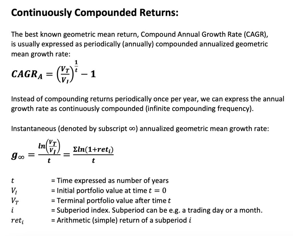
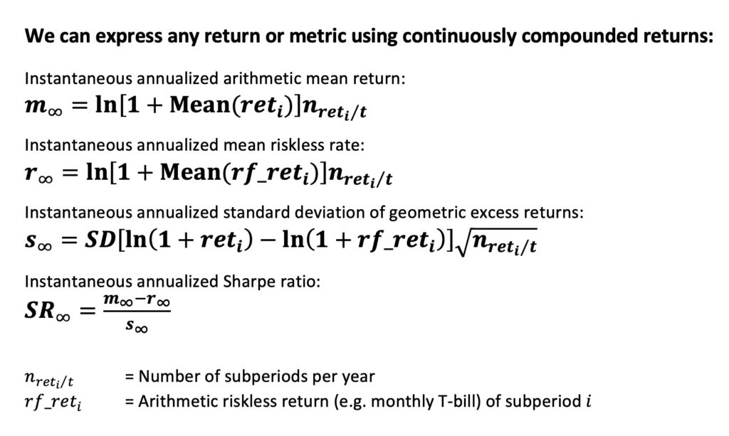
Furthermore, the formulas and results we show, all assume and use instantaneous i.e. continuously compounded rate of returns (log returns). Instantaneous means infinitely short time horizon implying no compounding has taken place. Continuous compounding means that instantaneous growth rate is compounded at infinite compounding frequency. All of our parameters are instantaneous. For example, Sharpe ratio uses instantaneous mean excess return and volatility of instantaneous excess returns instead of the original (as specified by Sharpe) mean compounded excess return and volatility of compounded excess returns. When using instantaneous rate of returns, the equations we show are exact. The big picture and conclusions will not change if we don’t use instantaneous rate of returns, but our formulas become (typically very accurate) approximations.

Note that the output of the formulas will always be expressed as instantaneous rate of return even if the inputs are not. See Appendix 1 for more information about continuously compounded returns and the transformation between continuously compounded rate of return and more commonly used annually compounded rate of return (CAGR).

Expected geometric excess return as a function of investment fraction

When the volatility of returns is higher than zero, expected geometric return is always lower than expected arithmetic return. In case of zero volatility, the two expectations are equal. There are many names for this phenomenon, e.g. volatility tax, variance drain or variance drag.

The equation of annualized expected geometric return (or excess return) is derived e.g. by Thorp [5] or in my thesis [7]. We show the formula below. First thing to notice that the investment fraction (risky asset allocation, f = 1 corresponds to 100% allocation) term in the variance drag is squared. This means that variance drag is very sensitive to risky asset allocation and increases quickly with leverage. Alternatively, we can express the annualized expected geometric excess return as a function of investment fraction, volatility and Sharpe ratio. We will see that Sharpe ratio is found everywhere when we explore the world of geometric returns and fractional Kelly criterion.

It is important to define parameters clearly. We can see that geometric Sharpe ratio is embedded in the formula. It is quite common in finance to see Sharpe ratio being casually replaced by geometric Sharpe ratio. These are two fundamentally different metrics: the former is based on arithmetic returns and is indifferent to investment fraction, the latter is based on geometric returns and therefore a (linearly descending) function of investment fraction.

The first derivate and the investment fraction leading to maximum annualized expected excess return is found by differentiating with respect to investment fraction. The first derivate gives us the marginal benefit of additional allocation to risky assets. The marginal benefit diminishes linearly.

We mentioned that Claude Shannon determined a mathematical upper bound – information channel capacity, the Shannon limit – for average error free information exchange rate over a noisy channel. The same mathematical upper bound applies to compounding process. We can determine compounding process capacity – the Shannon limit – as a mathematical upper bound for average compound excess growth rate of a risky investment. More about the Shannon limit can be found from my thesis [7] or (in more compact form) from this twitter thread [8].

Thinking in terms of compounding process capacity can be useful as it emphasizes the nature of the maximum attainable expected growth rate as a mathematical fact. A mathematical upper bound does not care and is not affected by the preferences, the utility function or the risk tolerance of a particular investor. This was also Kelly’s point as he pointed out that his formula has nothing to do with utility functions, but just reflects the mathematical fact that it is the logarithm of the returns which are additive and to which the law of large numbers applies to [4].

There is a way around the Shannon limit though: don’t compound your returns from period to next. This way you can enjoy arithmetic returns, which don’t utilize compounding process and therefore are not bounded by the compounding process capacity. The downside is that you can’t enjoy the benefits of compounding meaning you can’t grow your wealth exponentially over time.

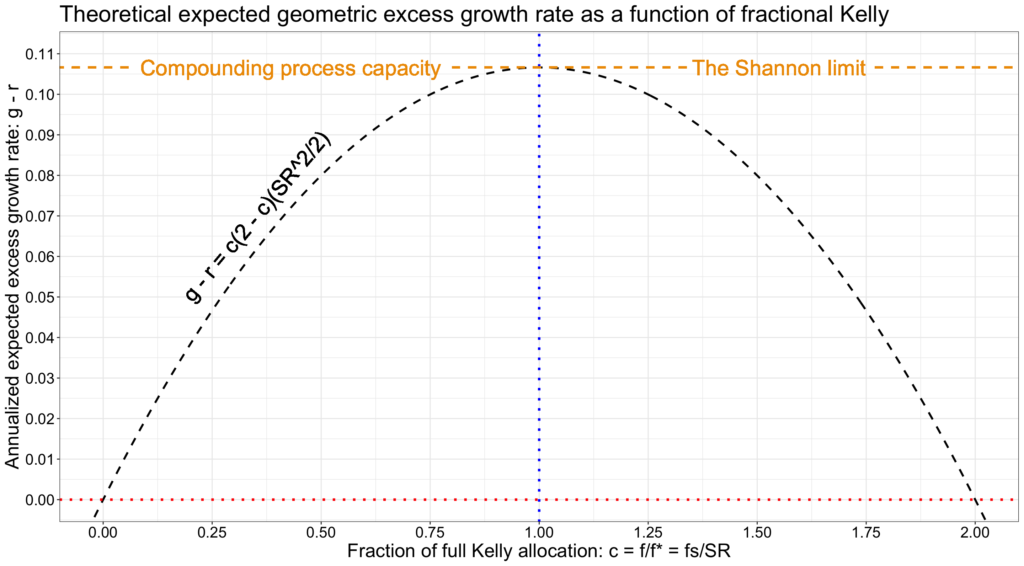
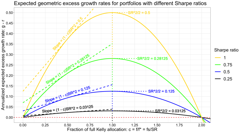
The shape of the expected geometric excess growth rate is a parabola as shown in the figure below. Zero expected excess growth rate equals expected riskless rate.

In the figure below, and in all figures except where otherwise stated, we use empirical parameters calculated based on daily excess returns (‘Mkt-RF’ in French data [9]) in the U.S stock market between Jul-1926 and Jun-2021.

The marginal benefit of additional allocation to risky assets is diminishing. The marginal benefit diminishes linearly and turns negative after full Kelly allocation, where the slope is zero.

Expected geometric excess return as a function of fractional Kelly

Instead of investment fraction, we can express the expected geometric excess return as a function of fraction of full Kelly allocation. Following Thorp [5], we call fraction of full Kelly allocation as fractional Kelly (e.g. “half Kelly” means half of full Kelly allocation). Thorp, and other advocates of the Kelly criterion, have been criticized (most notably by Paul Samuelson) that pursuing maximum expected growth rate at full Kelly allocation is too risky for most investors. I agree with this criticism and so does Thorp. Thorp emphasizes the use of fractional Kelly instead of targeting full Kelly (see e.g. [5] or [6]). In practice fractional Kelly means targeting an allocation between zero (all capital in riskless rate) and full Kelly, depending on our assessment on the reliability of the estimated parameters and our risk preferences. Negative allocation means shorting the risky portfolio, which may be profitable at times, but (thanks to risk premium) not a viable strategy (in the market level) for the long-term.

If we knew the market (sample) parameters (volatility and Sharpe ratio) of a given future time period, then we should target full Kelly to maximize the growth of our wealth. If we know the expected (population) parameters and invest a finite time period, then we may not want to target full Kelly as the outcome is uncertain and the confidence interval of our return distribution (depending on our time horizon) may be wide. And, in the realistic case that we don’t know the population parameters, it is very risky to target the allocation we think is the full Kelly allocation as if we go beyond full Kelly our expected growth rate starts to decrease. Even in the hypothetical best (the first) case, where we know the parameters which will realize for a given future period, there is a risk that large drawdowns will lead to ruin caused by forced liquidation or capitulation before the time period comes to an end.

The fractional Kelly criterion becomes incredibly simple and intuitive when we express the annualized expected geometric excess return as a function of fraction of full Kelly allocation. As shown below, we can decompose the expected geometric excess growth rate to two components: 1) a parabola, which is scaled by 2) the compounding process capacity expressed simply as half of squared Sharpe ratio. Not only the maximum (the Shannon limit), but the whole parabola is scaled by the compounding process capacity. This underlines the importance of maximizing the compounding process capacity, which is the same as maximizing the (square of) Sharpe ratio.

The first derivative gives us the instantaneous rate of growth rate change. The marginal benefit simplifies to two components: 1) a descending line, which is scaled by 2) the square of Sharpe ratio. The marginal benefit of additional allocation to risky assets is linearly diminishing. This means that with a given portfolio, additional allocation to risky assets is discouraged as the marginal reward is diminishing. This is as opposed to conventional finance theory, based on arithmetic returns, where the marginal reward is constant. Keeping the fraction of full Kelly allocation constant and comparing across alternative risky portfolios, the marginal reward is scaled by the square of Sharpe ratio. This means that doubling the Sharpe ratio quadruples the marginal reward of an additional allocation to risky assets. In conventional finance, doubling the Sharpe ratio doubles the marginal reward. In the world of geometric returns, Sharpe ratio is not only important, but important raised to the second power.

Expected growth rate is maximized at full Kelly allocation when the fraction of full Kelly allocation c = 1. Allocating only half of the full Kelly allocation, i.e. utilizing half Kelly allocation, yields exactly three quarters of the expected growth rate at full Kelly, but with only half of the volatility. Allocating 1.5 Kelly yields the same expected growth rate as half Kelly, but with three times the volatility. Furthermore, the fraction of full Kelly allocation c determines drawdown risk. See my post Drawdown risk = portfolio volatility normalized by Sharpe ratio (or shorter twitter thread [10]), where we show that c/2 corresponds to expected drawdown. We can therefore interpret that half Kelly yields three quarters of the expected growth rate of full Kelly with just half of the drawdown risk. At twice the full Kelly allocation (c = 2), expected excess growth rate is exactly zero equalling riskless rate. Beyond c = 2, expected excess growth rate is negative.

The marginal benefit diminishes linearly and turns negative after full Kelly allocation at c = 1, where the slope is zero.

Capital market parabola

Conventional finance theory advocates portfolio selection targeting maximum Sharpe ratio. Maximum Sharpe ratio is famously achieved by tangency portfolio i.e. the portfolio which forms a point of tangency on the Markowitz efficient frontier for the line drawn from riskless rate. The slope of the line is the Sharpe ratio.

By lending or borrowing (theoretically at riskless rate), the tangency line extends to as low or as high risky asset allocation as we like. The tangency line is called capital allocation line (CAL). Or, in the case that our risky asset portfolio is the market portfolio, the capital market line (CML). Important property of CAL and CML is that no other portfolio, formed in a given asset space, will have a higher reward (expected arithmetic excess return) with a given level of risk (volatility) or lower risk with a given level of reward. In other words, CAL and CML represent the most (mean-variance) efficient portfolios available.

Let’s demonstrate with three imaginary assets with known (realized) parameters for a given time period. The assets have different mean excess returns and especially volatilities. Correlations between assets are low, some slightly negative and some positive. The portfolio weights turn out to favour low volatility asset with these parameters. Importantly, no other portfolio formed using these three assets has a higher risk adjusted excess return (Sharpe ratio) than the tangency portfolio formed with the asset weights shown below.

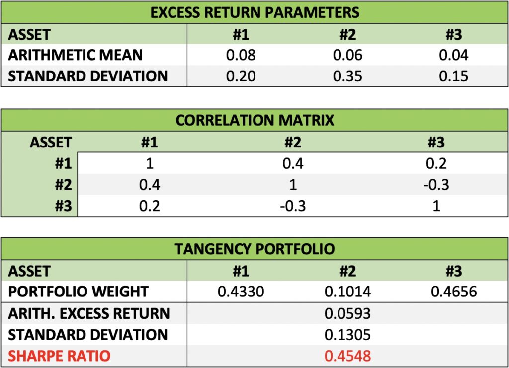
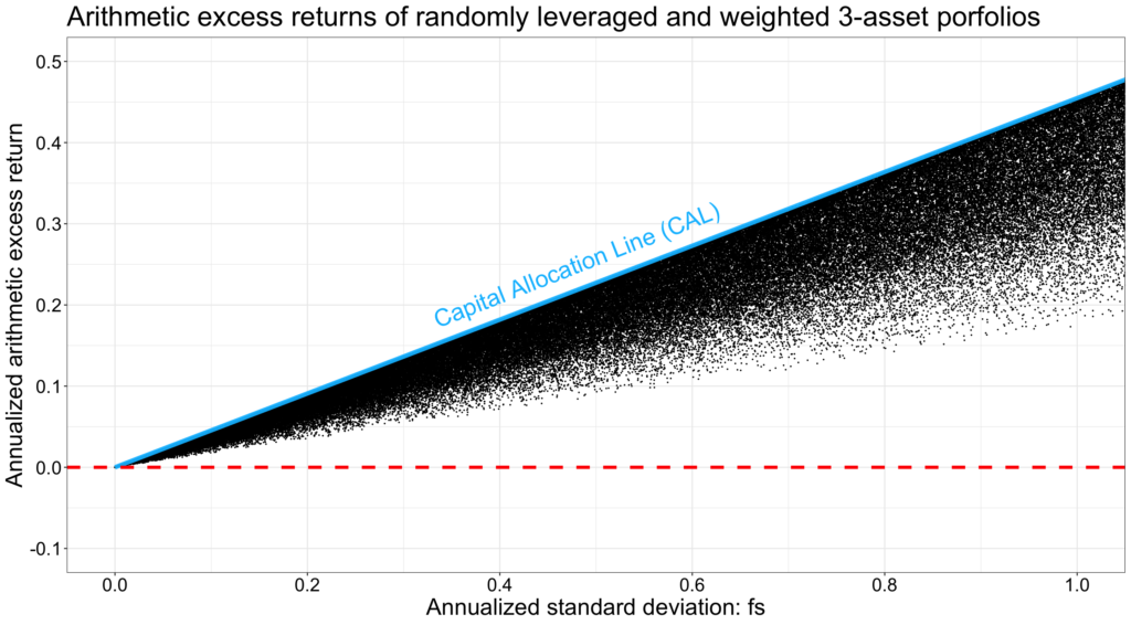
We can run a simulation utilizing our three assets with known parameters. We first create random asset weights (sum of weights = 1) for each portfolio and then leverage the portfolio randomly (random investment fraction). Keeping investment fraction positive, we see the returns as a function of portfolio volatility for tens of thousands of simulated random portfolios below. The figure speaks the language of capital efficiency. Capital allocation line represents our tangency portfolio combined with riskless rate (by lending or borrowing) and has its slope determined as the Sharpe ratio of the tangency portfolio: 0.4548. All of the randomly formed portfolios have an excess return lower than the tangency portfolio at a given level of portfolio volatility.

Capital allocation line and the capital market line in the market portfolio level are key concepts of finance theory. The fundamental principle of finance is – as can be seen from the figure below – that higher reward requires higher (systematic) risk. As long as you can tolerate the risk, only the sky (and availability of leverage) is the limit of your expected reward. Even the worst outcomes of our simulation don’t look too bad, they are always positive and rising with leverage. Seeing this figure, I am tempted to think that I can tolerate a whole lot of risk if the reward is as depicted here.

The reality of an investor living in the world with time and compound returns is – of course – very different from what is depicted by a single period model. Approximately symmetrical probability density function (PDF) around the CAL and the random arithmetic portfolio excess returns in the above figure is what you can expect if you invest multiple short-term periods and don’t reinvest your proceeds into the next period. Say, for example, that you invest $1000 every trading day (for a duration of one day) regardless your winnings or losses the previous day. If you want to earn interest on interest, then the arithmetic excess returns in the above figure don’t describe your typical returns anymore. As long-term investors want to grow their wealth exponentially over time, they care about – and the law of large numbers applies to – geometric (instead of arithmetic) returns. In the world of geometric returns, the manifestation of capital efficiency is the capital allocation parabola or, in the case that our risky asset portfolio is the market portfolio, capital market parabola. It is the very same parabola we just discussed in the context of fractional Kelly criterion. In the below figure we see the same random portfolios as in the previous figure but now expressed as geometric excess returns, which are bounded by the capital allocation parabola.

Leveraging up to infinite leverage – no matter what your risk tolerance is – does not look like such a good idea anymore. While the efficient portfolio is at its maximum excess return (SR^2/2 = 0.1034), the worst portfolios are losing to riskless rate. Not to mention that all portfolios lose to riskless rate when we exceed 2x full Kelly allocation. As shown mathematically and emphasized by Thorp [6], fractional Kelly criterion (represented here by the capital allocation parabola) represents the capitally efficient portfolios in the world of geometric returns. Capital allocation parabola represents the highest attainable reward (expected geometric excess return) with a given level of risk (volatility) or the lowest risk with a given reward. Portfolios are capitally efficient and on the rational frontier of the capital market parabola when 0 < c <= 1.

Note that even though expected growth rate (SR^2/2) is maximized globally at full Kelly allocation when Sharpe ratio is maximized, this is not the case generally. In case we don’t have full Kelly allocation, it is possible (with a given allocation to risky assets) to find portfolios with higher expected growth rate than the max Sharpe portfolio. It is, however, not possible to find portfolios with better expected excess growth rate / volatility trade-off than the max Sharpe portfolio.

In the above examples, with capital allocation line and parabola, all portfolios (with a given level of risk) lost to tangency portfolio. All portfolios will lose to tangency portfolio only when we know the realized returns and calculate the tangency portfolio after the fact (after the returns have realized), but not in the case when we only know the expected or predicted parameters and calculate the tangency portfolio based on those. Expectation is the mean value and there is a distribution around the mean.

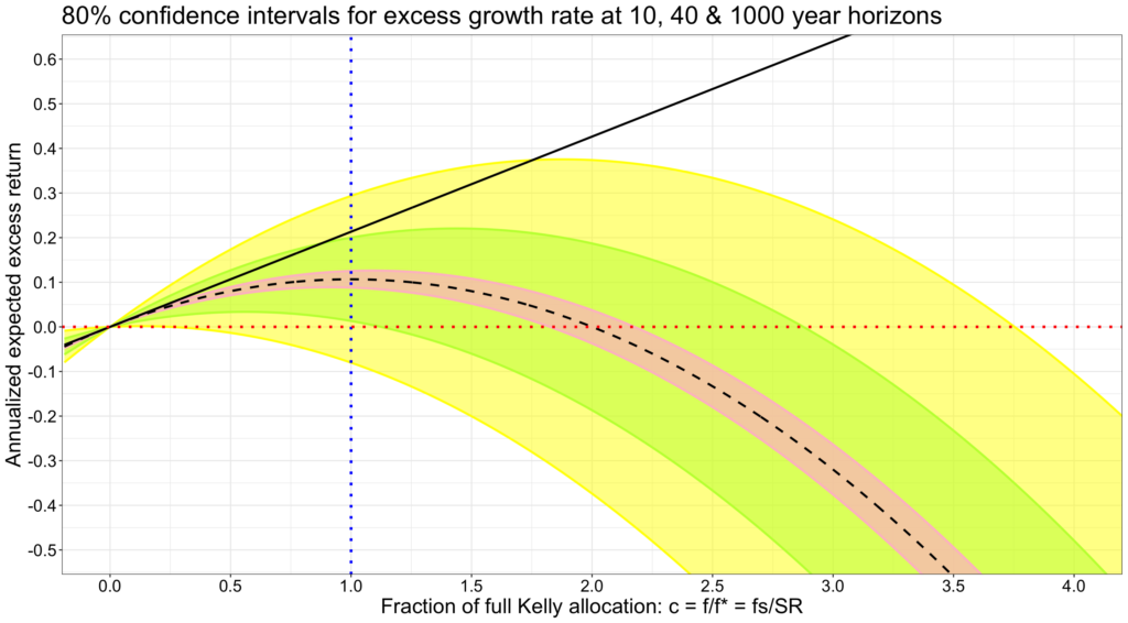
Let’s apply confidence intervals around the expected excess growth rate to illustrate how time and investment fraction play a role when we only know the expected parameters. It is well known – thanks to law of large numbers – that time narrows the distribution of annualized returns. Therefore, the confidence interval narrows closer to expected growth rate as time horizon increases. As we have learned, not only time, but investment fraction (or leverage) affects the distribution of returns. First of all, investment fraction increases the variance drag, and the impact is squared. Secondly, increasing investment fraction increases volatility in direct proportion. Of these two, the squared impact to variance drag of the expectation dominates the linear increase of volatility around the expectation. We assume normally distributed instantaneous geometric excess returns, which should be ok assumption in the long-term thanks to central limit theorem.

Below we see an 80% confidence interval around the expected excess growth rate (empirical U.S. daily data between Jul-1926 and Jun-2021). In other words, there is a 1/10 chance to exceed the upper bound of the confidence interval. The confidence interval is shown for three different time horizons. The longer the time horizon, the narrower the confidence interval and the more likely it is that the expected arithmetic excess return (capital market line) or higher will not realize. And particularly, the higher the allocation to risky assets, and therefore the higher the fraction of full Kelly allocation, the more likely it is that the return of CML or higher will not realize. For example, at 40-year horizon, there is about 10% chance that return of CML will be achieved at full Kelly allocation. And at 10-year horizon, there is about 90% chance to lose to riskless rate at 3.75 times full Kelly allocation.

Next figure has 99.8% confidence interval meaning that there is 1/1000 chance to exceed the upper bound. Give it 1000 years at 0.5 times the full Kelly allocation, 40 years at 2 times or 10 years and 4.25 times, and the chance of achieving the return of CML is about 1/1000. From the point of view of an individual investor enjoying compounded returns, given enough time and high enough allocation to risky assets, it is practically impossible to realize the return of CML. This is the case because of mathematics and regardless the risk tolerance of that particular investor.

Alternatively, we can illustrate the effect of time on arithmetic (capital market line) and geometric (capital market parabola) rates of returns using terminal wealth distributions after 10 years of compounding. The figure below (now with slightly different parameters) uses log-normal model implying normally distributed log returns. With log-normal model, median excess terminal wealth is exactly the wealth compounded using expected geometric rate of excess return as the growth rate. Now we have modelled riskless rate to be zero, meaning that excess terminal wealth = terminal wealth. Median terminal wealth (the blue line) finds its maximum at full Kelly allocation when investment fraction f = 2. The log-normally distributed probability density function (PDF) of terminal wealth shows how additional leverage turns the PDF more and more positively skewed and the bulk of the distribution including the mode (the most likely outcome, the black line) is pushed towards 100% loss. As allocation to risky assets increases, the arithmetic mean terminal wealth (the wealth compounded using expected arithmetic rate of excess return as the growth rate), shown as the red line, grows exponentially towards infinity. Simultaneously, the arithmetic mean terminal wealth becomes increasingly dependent on the rare favourable outcomes of the right tail and the probability of achieving or exceeding the arithmetic mean terminal wealth approaches (but never achieves) zero.

Considering the capital market parabola and the diminishing marginal benefit of additional allocation to risky assets, it is easy to understand why many investors are leverage averse. We could argue that, to some extent, it is rational to be leverage averse in the world of geometric returns. Understanding our approximate position on the parabola may help us make more informed decisions about our allocation to risky assets.

What Sharpe ratio really means?

What Sharpe ratio means? According to conventional finance theory, Sharpe ratio is mean arithmetic excess return (mean return in excess of mean risk-free rate) divided by the standard deviation of the excess returns. In other words, Sharpe ratio is risk adjusted excess return described as the amount of expected arithmetic return in excess of riskless rate per unit of risk. This is all correct and important, but not very tangible. We get a little bit closer to tangible when Sharpe ratio is described as the slope of the capital market line. But we really need to consider geometric excess returns to truly understand the meaning and implications of the Sharpe ratio.

Based on the formulas that we have shown earlier, all derived in [7], we can draw a Shape triangle. The Sharpe triangle, as shown in figure below, shows the capital market line (CML) as the hypotenuse of the triangle. Portfolio risk i.e. the standard deviation equals Sharpe ratio exactly at full Kelly allocation. This is shown as the horizontal cathetus of the Sharpe triangle and is also shown by Baz & Guo [11]. Finally, we can express the vertical cathetus as the square of Sharpe ratio, which is equal to expected arithmetic excess return and variance of geometric excess returns at full Kelly allocation. The rational frontier (0 < c <= 1) of the capital market parabola is bounded within the Sharpe triangle.

Whereas in conventional finance theory Sharpe ratio merely determines the efficient portfolio, in the world of geometric returns the whole rational opportunity set is determined and bounded by the Sharpe ratio. Note that the efficient portfolio maximising the Sharpe ratio is (practically) identical between the conventional finance theory (based on arithmetic returns) and the fractional Kelly criterion (based on geometric returns). This means that the actual portfolio selection across assets is identical. It is the portfolios travel across time which is different between arithmetic and geometric returns. Even though we emphasize that time averages should be used when considering compounded portfolio returns over time, it is important to keep in mind that we must use arithmetic returns in portfolio selection and asset pricing across assets. Arithmetic returns are additive across assets and assets are priced in relation to other assets.

In the context of geometric returns, we can define risk neutral compounder as an investor who only cares about maximizing his expected geometric return without considering the risk. Risk neutral compounder is equivalent to investor with logarithmic utility function. Risk neutral compounder has a strategy which consists of only two steps: 1) construct a portfolio which maximizes Sharpe ratio, 2) leverage the portfolio with volatility target = Sharpe ratio. Remarkably, in the world of geometric returns, risk neutral compounder only considers two metrics: Sharpe ratio and volatility. How different is that from the world of arithmetic returns where risk neutral investor considers only expected return.

Most of us are not risk neutral and care about the risk too. Such risk averse compounders can find a capitally efficient portfolio from the rational frontier of the capital market parabola by targeting volatility <= Sharpe ratio. Doing so they give up some expected growth rate, but gain lower risk and higher risk adjusted growth rate.

How risky full Kelly allocation then is? As shown in post Drawdown risk = portfolio volatility normalized by Sharpe ratio, full Kelly allocation means that your drawdown probability density function is a continuous uniform distribution. This means that any drawdown is equally likely. A drawdown of 0% to 1% is equally likely with a drawdown of 99% to 100%. You can imagine the amount of uncle points met at full Kelly allocation. And in reality, the parameters determining full Kelly allocation are uncertain estimates, making it even more risky to target full Kelly.

In the figure below, we compare portfolios with different Sharpe ratios. The maximum rational volatility for a compounder is equal to Sharpe ratio. We can see how the half of square of the Sharpe ratio – the compounding process capacity – scales the opportunity set, the capital allocation parabola.

The next figure shows risk as fraction of full Kelly allocation c. We can think this as having the same drawdown risk (c/2 is the expected drawdown) across portfolios with different Sharpe ratios and compare the expected excess growth rate opportunity sets (capital allocation parabolas). First thing to notice is that the difference between the maximum attainable expected excess growth rates is the difference between half of squared Sharpe ratios. Doubling the Sharpe ratio means quadrupling the maximum expected excess growth rate. Quadrupling Sharpe ratio means 16x the maximum growth rate. The same squared Sharpe relation applies to marginal reward. It is much more beneficial to take on more drawdown risk with high Sharpe portfolio compared to low Sharpe portfolio. Increasing the risky asset allocation with a SR = 1 portfolio has a 16x higher increase in expected growth rate per unit of increased drawdown risk compared to portfolio with SR = 0.25.

Empirical results

We have shown how the fractional Kelly criterion works in theory. Theory has little value if it is not applicable in practice. We can test the fractional Kelly criterion with empirical data. We use empirical daily excess returns (‘Mkt-RF’ in French data [9]) in the U.S stock market between Jul-1926 and Jun-2021. 

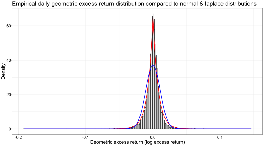
The figure below shows that daily empirical instantaneous geometric excess returns (excess log returns) are not normally distributed (blue line), but instead closely follow the shape of the fat tailed Laplace distribution (red line). In addition, empirical daily returns are slightly negatively skewed and the geometric mean corresponds to 47.4 percentile instead of the 50 percentile (median). See more about Laplace distribution and empirical returns e.g. from Harwood [12].

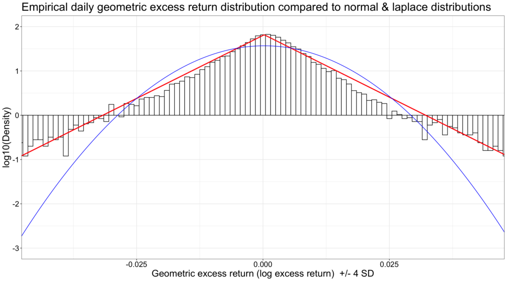
By transforming the y-axis to logarithmic and showing the +/- 4 standard deviation range, we can see how the tails are a much better match with Laplace than normal distribution. 

The figure below shows both the theoretical (based on metrics calculated from the empirical data) and empirical annualized mean excess growth rate. Riskless rate is monthly T-bill rate. Remember that we always use instantaneous metrics. Instantaneous empirical annualized Sharpe ratio is 0.4618 and annualized volatility of instantaneous excess log returns is 0.1751. For comparison, conventional annualized Sharpe ratio is 0.4626 and annualized volatility of excess returns is 0.1749. The difference between instantaneous metrics and conventional metrics in this case is negligible.

Empirical full Kelly allocation is f* = 2.59 (corresponding to 259% stock allocation) compared to theoretical value f* = 2.64. Maximum leveraged annualized mean excess growth rate at full Kelly allocation is 0.1059 compared to theoretical value of 0.1066. 100% stock allocation corresponds to c = 0.38 i.e. 38% of full Kelly allocation, which corresponds to theoretical value. Annualized mean excess growth rate at f = 1 is 0.0656, which corresponds to theoretical value. The relevant range for rational compounder is 0 < c <= 1. In this range, empirical capital market parabola corresponds to its theoretical counterpart extremely accurately. 

In the range c > 1, empirical annualized mean excess growth rate starts to increasingly lag the theoretical value. The reason is a combination of less than infinite (daily) rebalancing frequency and fat tailedness of the daily return distribution. Empirical stock market is closed at nights and weekends. Theoretical formula for fractional Kelly criterion assumes continuous returns and rebalancing back to target investment fraction with infinite frequency. Nevertheless, we can consider empirical values to closely follow theoretical prediction even close to c = 2.

What if we rebalance monthly instead of daily? We can test monthly rebalancing empirically by using monthly data from the same time period. Let’s use empirical monthly excess returns (‘Mkt-RF’ in French data [13]) in the U.S stock market between Jul-1926 and Jun-2021. We can see from the figure below that monthly rebalancing frequency is not high enough at high levels of risky asset allocation.

Instantaneous empirical annualized Sharpe ratio is 0.4453 and annualized volatility of instantaneous excess log returns is 0.1853. For comparison, conventional annualized Sharpe ratio is 0.4473 and annualized volatility of excess returns is 0.1851. The difference between instantaneous metrics and conventional metrics is very small.

100% stock allocation corresponds to c = 0.42 compared to 0.38 with daily rebalancing. Theoretical full Kelly allocation f* = 2.40 compared to 2.64 with daily rebalancing. Empirical full Kelly allocation f* = 2.20. Maximum leveraged annualized mean excess growth rate at full Kelly allocation is 0.0957 compared to theoretical value of 0.0991.

Monthly rebalancing frequency is enough for empirical fractional Kelly criterion to match accurately with theoretical prediction on the rational frontier of the parabola up to close to full Kelly allocation. Theoretical capital market parabola is the upper bound and the importance of empirical rebalancing frequency becomes the more important the higher the risky asset allocation. Compared to daily, with monthly rebalancing the difference between theoretical and empirical parabola is larger at the top and particularly on the decreasing frontier of the parabola. Approaching and especially exceeding full Kelly allocation with too low rebalancing frequency is even more risky than the theory (based on infinite rebalancing frequency) predicts.

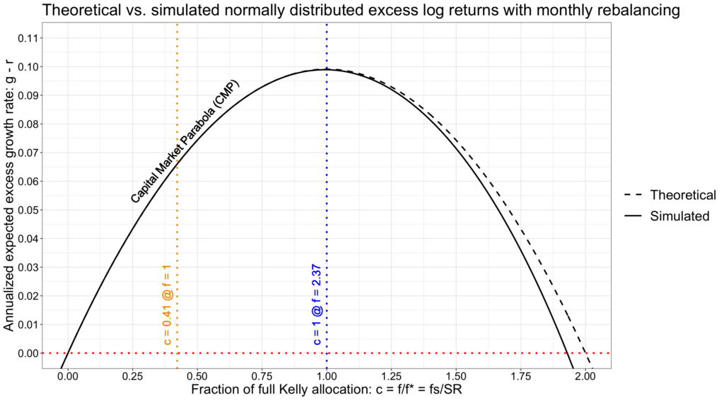
To find out the effect of fat tailed autocorrelated returns, we can compare the above monthly rebalanced empirical parabola to figure below, where we have simulated a parabola by drawing random log-normally distributed monthly excess returns (implying normally distributed excess log returns). Monthly returns mean monthly rebalancing to target risky asset allocation. To have a fair comparison, we use the realized empirical parameters as population parameters in simulation and select (among many trials) the realized simulation which parameters match closely with realized empirical parameters. Instantaneous simulated annualized Sharpe ratio is 0.4452 and annualized volatility of instantaneous excess log returns is 0.1879.

With normally distributed excess log returns we don’t have fat tails or autocorrelation and monthly rebalancing is enough to keep the difference between theoretical and simulated parabola practically non-existent before we are clearly over the full Kelly allocation. There is a small difference as we get closer to 2x full Kelly allocation. 

We conclude that, with historical U.S. market parameters, when on the rational frontier of the parabola and given high enough – say daily – rebalancing frequency, theoretical fractional Kelly criterion accurately predicts empirical long-term results and is robust against skewness, fat tailedness (excess kurtosis) and the well documented autocorrelation of empirical daily geometric excess returns. However, approaching and exceeding full Kelly allocation is very dangerous especially if portfolio is not rebalanced very frequently. With monthly rebalancing, theoretical maximum excess growth is not achieved and exceeding full Kelly allocation leads to deteriorated expected excess growth rate much quicker than theory predicts. The higher the allocation to risky assets – in practice, the higher the leverage – the more important frequent rebalancing back to target risky asset allocation becomes.

Conclusions and implications

Geometric expectation over time is the expected portfolio growth rate when returns are reinvested and compounded. This applies to portfolio returns – after reaching the limits of diversification – over time. Arithmetic expectation over an ensemble is the expected return for repeated or parallel single period bets. Of these two, geometric expectation describes the typical outcome for a long-term investor with only life to live and invest.

The difference between arithmetic (ensemble) average and geometric (time) average is the variance drag, which drags geometric average lower compared to arithmetic average. Variance drag is a squared function of risky asset allocation, which means that high (eventually leveraged) allocation to risky assets will lead to decreasing and eventually negative expected growth rate.

The great majority of long-term investors want to grow their wealth exponentially by compounding their returns. Geometric instead of arithmetic expectation therefore is the relevant metric at portfolio level for most long-term investors.

The Kelly criterion determines the risky asset allocation which leads to maximum expected logarithm of wealth (geometric expectation), which is different from expected wealth (expected value of the wealth i.e. arithmetic expectation). Full Kelly allocation is achieved when portfolio volatility is equal to the Sharpe ratio of the portfolio.

Fractional Kelly criterion determines capital market parabola, which is the geometric world counterpart to capital market line determining capitally efficient portfolios.

Capital market parabola is determined by: investment fraction, volatility and Sharpe ratio, or alternatively: fraction of full Kelly allocation and half of square of Sharpe ratio.

Rational frontier (the increasing part) of the capital market parabola is bounded by the Sharpe triangle. Sharpe ratio determines not only the efficient portfolio, but the whole rational opportunity set in the world of geometric returns.

One half of squared Sharpe ratio is the compounding process capacity, the mathematical upper bound for average compound excess growth rate of a risky investment. Compounding process capacity – the Shannon limit – is the finance world counterpart to the famous information channel capacity determined by Claude Shannon.

Compounding process capacity scales the parabola implying that not only the maximum expected excess growth rate, but the whole rational frontier (opportunity set) of the parabola is scaled by the half of squared Sharpe ratio.

Marginal benefit of marginal additional allocation to risky assets as a function of fraction of full Kelly allocation is a descending line scaled by squared Sharpe ratio. With a given portfolio, additional allocation to risky assets is discouraged by the linearly diminishing marginal benefit. Across portfolios, keeping drawdown risk constant, the attractiveness of additional allocation to risky assets increases in squared relation to the ratio of portfolio Sharpe ratios. Additional allocation to risky assets is four times more attractive with a 0.6 Sharpe ratio portfolio compared to 0.3 Sharpe ratio portfolio.

In the world of geometric returns, Sharpe ratio is often squared and is even more important and restricting parameter than in the world of arithmetic returns.

We emphasize using geometric returns and fractional Kelly criterion when considering portfolio returns compounded over time. However, portfolio selection across assets must use arithmetic returns. Portfolio selection in the context of fractional Kelly criterion maximize Sharpe ratio and is no different from conventional finance theory. Shortly: arithmetic returns for assets (assets form a portfolio, no time aspect), geometric returns for portfolio (one portfolio consisting of potentially many assets compounds over time).

The law of large numbers applies to geometric excess returns and in the long run the probability of achieving the expected arithmetic excess return or higher approaches (but never achieves) zero. The higher the allocation to risky assets, the more quickly the probability approaches zero.

Theoretical capital market parabola is the upper bound of risk adjusted geometric expected rate of excess return. On the rational frontier of the parabola and with daily rebalancing, empirical fractional Kelly criterion very closely follows theoretical prediction. Given high enough rebalancing frequency, Kelly criterion is robust empirically, does not make assumptions on return distribution and tolerates return autocorrelation.

Monthly rebalancing frequency is sufficient until close to full Kelly allocation, but is not enough to guarantee expected excess growth rate predicted by theory at or higher than full Kelly allocation. Rebalancing is the more important the higher the allocation to risky assets. In practice, increasing leverage requires increasing rebalancing frequency.

The strategy of a risk neutral compounder consists of only two steps: 1) construct a portfolio which maximizes Sharpe ratio, 2) leverage the portfolio with volatility target = Sharpe ratio. In the world of geometric returns, risk neutral compounder only considers two metrics: Sharpe ratio and volatility.

Risk averse compounder will give up some expected growth rate and will target a volatility lower than Sharpe ratio. By doing so, risk averse compounder will have both lower risk and higher risk adjusted growth rate compared to choosing higher allocation on the rational frontier of the capital market parabola.

References

[1] Peters, O. (2019). The ergodicity problem in economics

[2] Shannon, C. E. (1948). A Mathematical Theory of Communication

[3] Poundstone, W. Fortune’s Formula: The Untold Story of the Scientific Betting System That Beat the Casinos and Wall Street

[4] Kelly, J. L. (1956). A New Interpretation of Information Rate

[5] Thorp, E. O. (2006). The Kelly criterion in blackjack, sports betting and the stock market

• For instantaneous geometric expected return, see derivation of eq. 7.2

[6] Thorp, E. O. (2008, May and September). Understanding the Kelly criterion. Wilmott magazine, columns from the series A mathematician on Wall Street.). KELLY CAPITAL GROWTH INVESTMENT CRITERION

[7] Kurtti, M. T. (2020). How many stocks make a diversified portfolio in a continuous-time world?

• 3.1.1     Single period versus continuous-time world
• 3.2        Derivation of instantaneous geometric expected excess return (geometric risk premium)
• 3.3.4     Kelly criterion and the magic of Sharpe ratio
• 3.3.5     The Shannon limit as a function of square of Sharpe ratio

[8] Kurtti, M. T. (2022). Twitter thread: The Shannon limit

[9] Kenneth French. ‘Fama/French 3 Factors [Daily]’ Kenneth French data library

[10] Kurtti, M. T. (2022). Twitter thread: What determines drawdown depth?

[11] Baz, J. & Guo, H. (2017). An asset allocation primer: Connecting Markowitz, Kelly and risk parity. (PIMCO quantitative research).

[12] Vance Harwood. Predicting Stock Market Returns—Lose the Normal and Switch to Laplace

[13] Kenneth French. ‘Fama/French 3 Factors’ Kenneth French data library

Appendix 1

For the sake of simplicity, we have dropped the infinity subscript (which is used below to denote continuously compounded returns) from our formulas in the main body of this blog post.

Article by Markku Kurtti