
Long-term investors measure growth rate, but eat compound wealth.
The four determinants of terminal wealth ratio (randomly selected portfolio’s terminal wealth divided by benchmark terminal wealth) and probability of losing to fully diversified benchmark will be introduced and analyzed: Idiosyncratic variance of a single stock (idiosyncratic variance of the selected investing style), time horizon length, stock allocation (or leverage multiplier) and number of stocks in the portfolio.
Equations utilizing the four determinants will be derived and tested empirically. These relatively simple mathematical models are shown to predict empirical results accurately.
In short, we will show how compounding over time – an aspect largely absent in the conventional finance theory – needs to be considered to truly materialize and reveal the importance of diversification.
The math behind the diversification effect
In my earlier article, Diversification is a negative price lunch, we introduced two important concepts: diversification premium and diversification premium difference to benchmark. Diversification premium is the difference between the expected geometric growth rate of a (randomly selected) portfolio and the expected geometric growth rate of a (randomly selected) single stock portfolio. Diversification premium is always positive. Diversification premium difference to benchmark is defined as diversification premium difference between less than perfectly diversified portfolio and fully diversified benchmark portfolio. Diversification premium difference to benchmark is always negative.
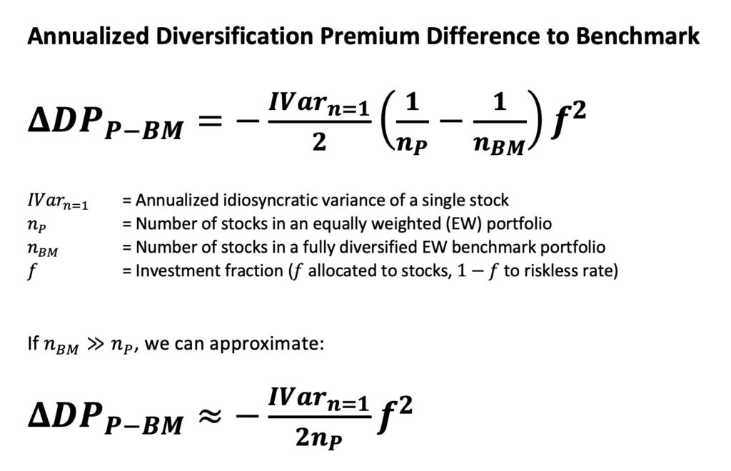
Equation of annualized diversification premium difference to benchmark for equally weighted portfolios and its approximate version are given below. Derivations can be found from section 3.3.1 in my thesis [1].
Annualized idiosyncratic variance of a single stock is estimated from data. Notice that empirical number of stocks in the benchmark can vary from month to month (or day to day, depending on the frequency of the data). As diversification premium is essentially a growth rate, we want to keep the weight of each month (or each time instant) equal. To achieve equal weight for each time instant, we need to compensate for the differences in number of stocks per time instant when we estimate idiosyncratic variance of a single stock. The method how to compensate for the difference in number of stocks is given in section 3.3.2 in my thesis [1].
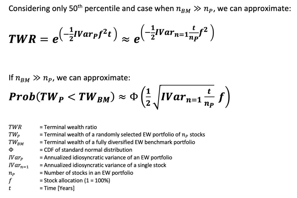
To be able to measure the effect of diversification on wealth instead of growth rate, we define terminal wealth ratio (TWR) as portfolio’s terminal wealth percentile divided by fully diversified benchmark portfolio terminal wealth. TWR is a function of diversification premium difference to benchmark. The equation of TWR for randomly selected equally weighted portfolios is derived and given below.
Note that our equations assume continuously compounded returns without jumps in prices with rebalancing back to equal weights and target stock allocation at infinite frequency. This means that our TWR equation presents theoretical upper bound and we can expect empirical TWR to be somewhat lower as empirical portfolios have lower rebalancing frequencies and returns are not continuous (markets are not always open).

Additionally, we derive the equation of probability of randomly selected portfolio losing to fully diversified benchmark for equally weighted portfolios.

To get intuitive understanding of the equations, we derive approximate versions below. These approximate versions work very accurately as long as the number of stocks in the portfolio is much lower than the number of stocks in the benchmark portfolio. It is very clear from these approximate equations that there are four determinants for both terminal wealth ratio and the probability of losing to fully diversified benchmark: 1) idiosyncratic variance of a single stock (idiosyncratic variance of the selected investing style or benchmark), 2) time horizon length, 3) stock allocation (or leverage multiplier) and 4) number of stocks in the portfolio. Determinants from 1 to 3 decrease terminal wealth ratio and increase the probability of losing to benchmark while the fourth determinant – diversification – works the other direction against the three other determinants. The impact of the third determinant, leverage multiplier, is particularly important as its impact is squared.
We can immediately see some interesting relations between the determinants. For example, to keep TWR and the probability of loss constant (to prevent TWR from decreasing and probability of loss from increasing) we need to increase diversification approximately in direct proportion to increase in time horizon length. In other words, – against the conventional wisdom – diversification becomes the more important the longer the time horizon. And to keep TWR and the probability of loss constant, we need to increase diversification approximately in squared proportion to increase in leverage multiplier. If there is one condition when diversification is important, it is when leverage is applied. Finally, to keep TWR and the probability of loss constant, we need to increase diversification approximately in direct proportion to increase in idiosyncratic variance of a single stock when we consider different investing styles (different benchmarks).
Illustrating diversification effect in the context of compound wealth
Next, we illustrate how compound terminal wealth is affected by the four determinants derived above and how the benefits of diversification fully materialize only after considering diversification in the context of compound wealth.
There are two important theorems, which explain why randomly picked portfolio growth rate distribution and – after compounding – terminal wealth (TW) distribution approaches the shape of normal and log-normal distribution, respectively. The first theorem is the law of large numbers (LLN), which describes how the average of a random sample converges towards its expectation as the number of independent trials increase. For more about LLN, see e.g. [2]. Second theorem is the central limit theorem (CLT). CLT describes how the sample means of randomly selected (large enough) samples converge towards the shape of normal distribution regardless the shape of the distribution where the samples are drawn from. For more about CLT, see e.g. [3].
Importantly, in the case of compound returns, LLN applies to logarithmic (instead of simple) returns. Logarithmic returns (natural logarithm of one plus simple return), which are additive over time, are geometric returns while simple returns are arithmetic returns. In other words, LLN applies to the mean geometric (instead of arithmetic) growth rate, which converges towards its expectation as the sample size increases i.e. as the time horizon length (the number of e.g. monthly logarithmic returns) increases.
Equally importantly, CLT applies to logarithmic (instead of simple) returns, which we can sum over time. In other words, CLT applies to samples of mean geometric growth rates resulting to sample mean growth rate distribution, which approaches the shape of normal distribution as the sample size increases i.e. as the time horizon length increases.
Note that the growth rates we use are all continuously compounded geometric returns, which ensures that our equations are mathematically exact.
The format of the illustrative figures below is adapted from [4].
It is well known that short-term stock market returns are not normally distributed, but have fat tails. The figure below shows how we start from a non-normally distributed short-term return distribution and sum (randomly selected) short-term logarithmic returns over time. It is the additivity of logarithmic returns which allows both LLN and CLT to work their magic and, over time, turn our long-term terminal wealth growth rate distribution approximately normally distributed with a mean approaching the expected terminal wealth growth rate. Both LLN and CLT work for sums of logarithmic returns, which are essentially sample mean growth rates for the given time period.
Note, however, that we need to (randomly) re-select the stocks in the portfolio frequently enough to get representative sampling across the cross-section of stock returns. If we hold each stock for years or decades, we may not get representative cross-sectional sampling even if the time horizon is long. Cross-section of stocks includes many different styles of stocks (big stocks, small stocks, micro caps, value stocks, growth stocks etc.). Historically different styles have had different mean returns, which (among other things) increases idiosyncratic variance of a single stock when we consider the whole population of stocks. With random sampling, terminal wealth ratio or probability of losing to benchmark can’t see the potential differences in mean returns though, they only see one interesting statistical parameter: idiosyncratic variance.
Notice from the figure below how the mean terminal wealth growth rate is materially lower (due to variance drag) for less than perfectly diversified 1-stock portfolio compared to fully diversified benchmark portfolio. And, of course, the variance of 1-stock portfolio is much higher compared to benchmark.
Compounding applied to approximately normally distributed terminal wealth growth rate transforms the terminal wealth distribution approximately log-normally distributed with common mean for all portfolios regardless the level of diversification, but materially lower median terminal wealth for 1-stock portfolio compared to benchmark (equally weighted market portfolio). And it is not only median, but also the mode (the most likely outcome) and the bulk of the 1-stock portfolio, which are materially lower compared to benchmark. 1-stock portfolios have a very long right tail (the lucky outcomes), which ensures that the mean terminal wealth is equal to benchmark mean.

For any given time horizon length, we have only one realized terminal wealth for the fully diversified benchmark portfolio and a large number of possible terminal wealths for less than perfectly diversified randomly selected portfolios. We have defined terminal wealth ratio (TWR) as (randomly selected) portfolio’s terminal wealth percentile divided by fully diversified benchmark portfolio terminal wealth. Next, we will consider terminal wealth growth rate and how compounding transforms it to terminal wealth ratio.
Importantly, when we consider terminal wealth ratio instead of terminal wealth, we only care about idiosyncratic variance. In case of terminal wealth, variance is the sum of systematic (non-diversifiable) and idiosyncratic (diversifiable) variance. But in case of TWR, we only need to consider cross-sectional terminal wealth variance, which is purely idiosyncratic.
As systematic time-series variance is absent from TWR analysis, it also means that the well-known time-series autocorrelation (mainly time-series momentum) of systematic (benchmark) returns is absent too. This is potentially important because autocorrelation can make CLT less efficient. We have a reason to assume that CLT will work more efficiently for terminal wealth ratio than for terminal wealth. In other words, we have a reason to expect approximately normally distributed TWR growth rates and approximately log-normally distributed TWR with empirical data regardless the well-known time-series momentum present in benchmark returns.
We can see from the figure below how annualized diversification premium difference to benchmark (essentially annualized variance drag difference between our portfolio and benchmark) multiplied by time compounds to median terminal wealth ratio.

Notice that the benchmark portfolio in our illustrations always shares exactly the same parameters with the portfolio we are examining except for one parameter: number of stocks in the portfolio.
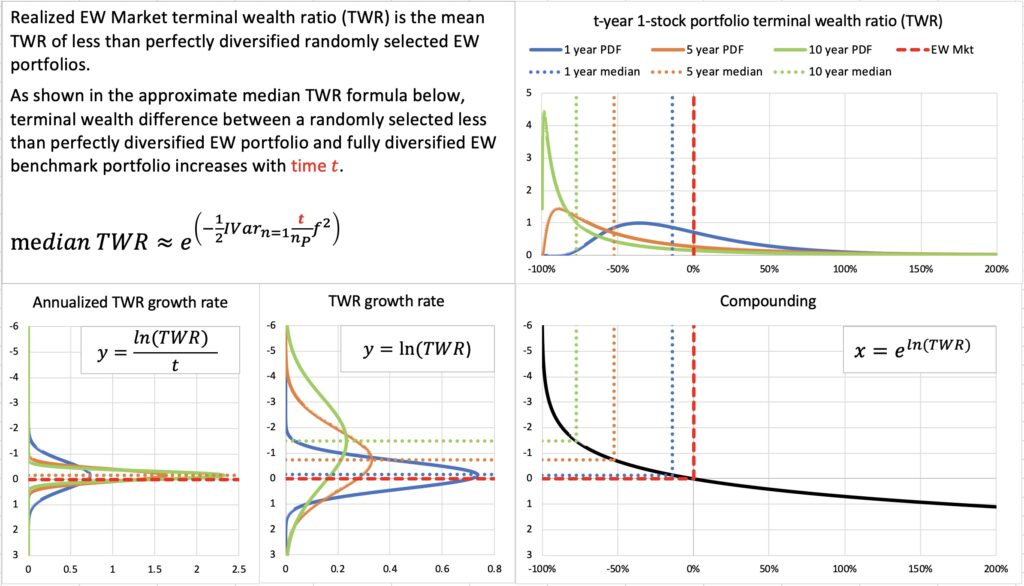
In the figure below, we illustrate the effect of time on terminal wealth ratio. Realized EW Market terminal wealth ratio is the mean TWR for less than perfectly diversified randomly selected EW portfolios. The difference between portfolio’s mean (EW Mkt TWR) and median TWR increases with time.
Compared to previous figure, we now show also annualized growth rate, which is typically the focus of analysis in conventional finance theory. Standard deviation of annualized TWR growth rate decreases with time, which in conventional analysis is often interpreted to mean that risk decreases with time. However, based on TWR growth rate and eventually TWR distribution, we can see that the mode and median TWR decrease and the probability of losing to benchmark actually increases with time. In other words, judged based on terminal wealth distribution (instead of annualized growth rate distribution), we find that risk increases with time.
Increasing diversification reduces idiosyncratic variance drag, which increases portfolio’s diversification premium and decreases diversification premium difference to benchmark.
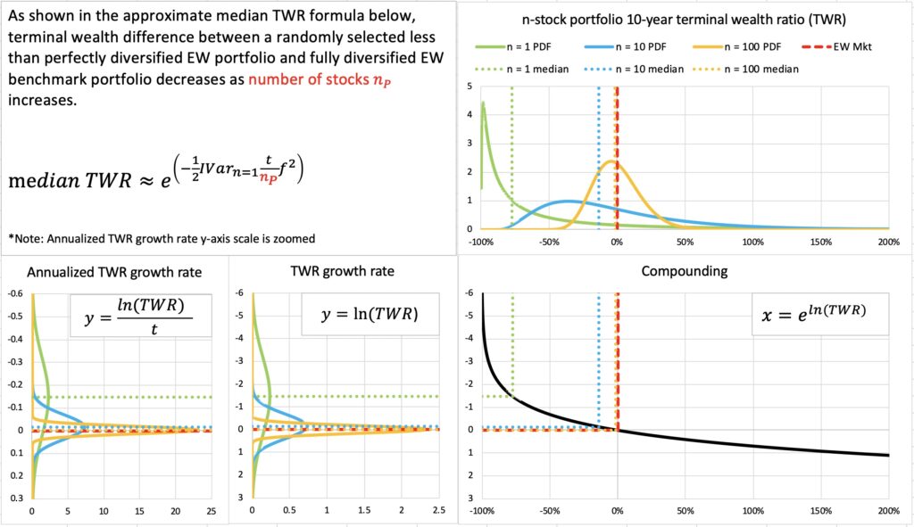
Idiosyncratic variance increases in direct proportion to time and decreases approximately in inverse proportion to number of stocks. To prevent median TWR from decreasing and probability of losing to benchmark from increasing, we need to increase diversification approximately in direct proportion to time. In the figure below, where we can see how the skewness of a 10-year terminal wealth ratio is greatly reduced as the number of stocks in our portfolio is increased. The dismal 10-year median TWR of a 1-stock portfolio is approximately the same what we expect to see for a 10-stock portfolio in a 100-year period.
In the absence of stock picking skill, diversification becomes the more important the longer the time horizon.
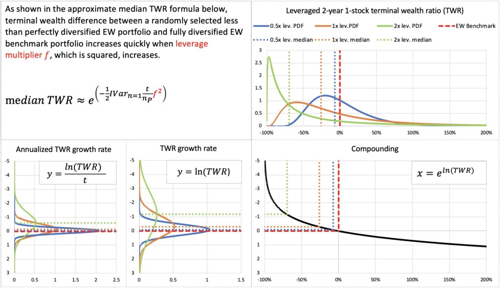
Idiosyncratic variance drag, and therefore (the magnitude of) diversification premium difference to benchmark, increases in direct proportion to time, but in squared proportion to leverage multiplier. The quickest way to drive median TWR low and probability to lose to benchmark high is increasing leverage. This is demonstrated in the figure below, where we have a short 2-year time horizon, but highly leveraged portfolio quickly decimates median terminal wealth ratio. On the other hand, low allocation to stocks manages to keep median TWR close to one.
In the absence of significant stock picking skill, diversification becomes the more important the higher the allocation to stocks.
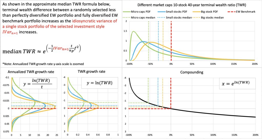
Finally, different investing styles come with different idiosyncratic variances. In the figure below, 40-year median TWR of a 10-stock portfolio is the lowest for micro caps, which are known to be loaded with idiosyncratic variance.
The importance of diversification is a function of selected investing style.
Empirical tests
Next, we test our equations empirically.
CRSP data
Our first test utilizes monthly CRSP data from Jan-1973 to Jun-2018. The data includes all common stocks (CRSP share codes 10, 11 and 12) from U.S. market. Delisting returns are included. In addition, we use annual Compustat accounting data to e.g. filter accounting based investing styles. More details about empirical tests with different investing styles can be found from section 5.8 in my thesis [1]. The reason why we don’t use longer data (starting from Jan-1926) is that CRSP data from Jan-1926 to present includes three distinct stock populations with very different characteristics (this is shown in section 4.1.1 in my thesis [1]). We focus on the latest period, which comprises of all three major stock exchanges in the U.S.: NYSE, NYSE Amex and Nasdaq.
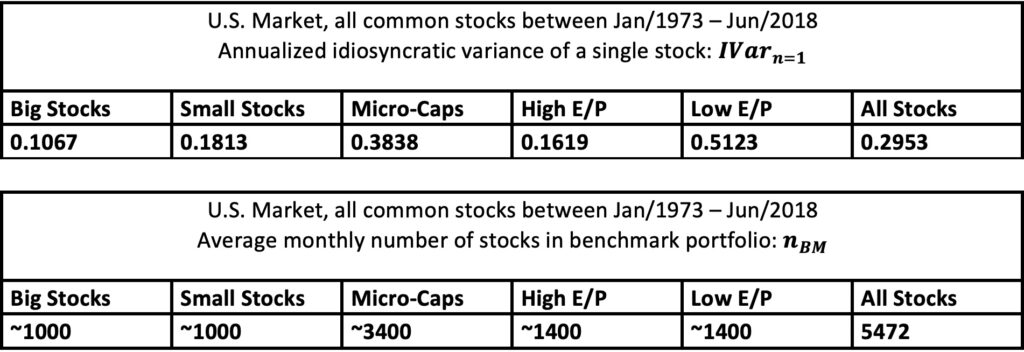
Tables below show idiosyncratic variances for single stock portfolios and average number of stocks per month estimated from empirical data. Data for “All Stocks” is used in this article (including illustrative figures in previous section) when not otherwise stated.
First, we test how effectively central limit theorem works with our empirical data. We use monthly excess returns i.e. returns in excess to monthly T-bill return (terminal wealth ratio and probability of losing to benchmark are the same regardless if we use returns or excess returns).
In our empirical tests we create 50 000 equally weighted portfolios randomly each month (monthly rebalancing) leading to 50 000 parallel return histories for different portfolio sizes (1, 10, 25 and 100 stocks) each extending 45.5 years. Random portfolios are created monthly by bootstrapping without replacement. The data consist of all stocks.
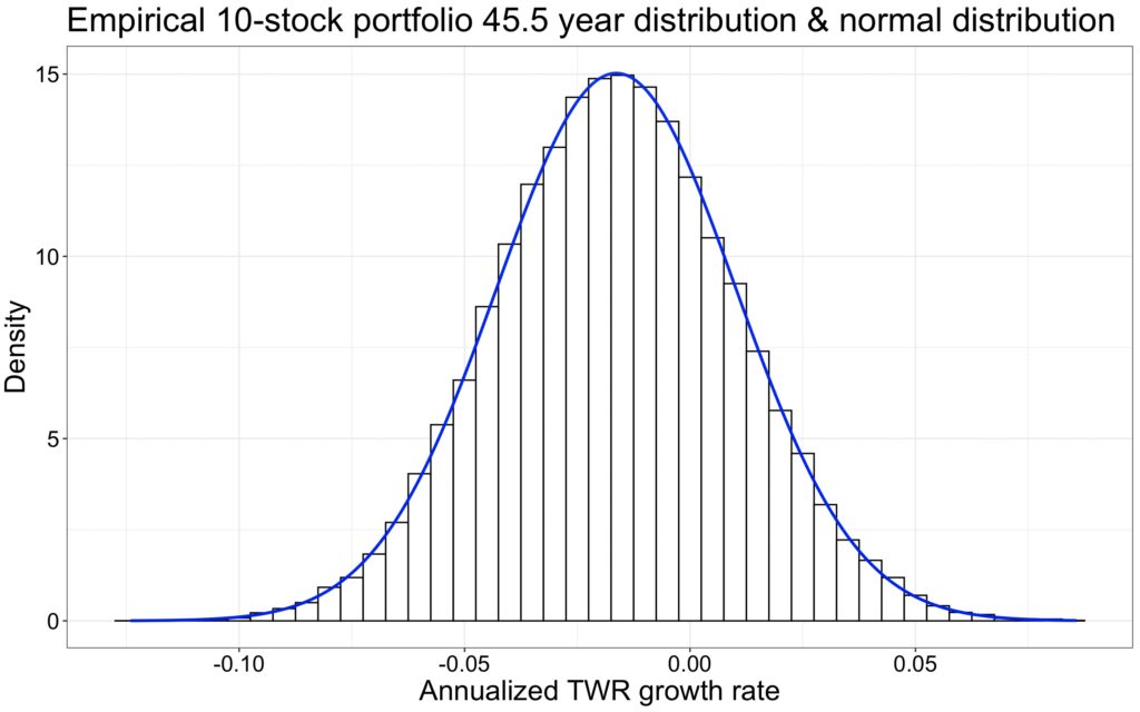
To demonstrate CLT, we use 10-stock portfolio test. If CLT works, our 45.5-year period TWR growth rate is normally distributed. In the figure below, we can see theoretical annualized TWR growth rate distribution (blue line) created using empirical parameters and empirical annualized TWR growth rate distribution (bar blot). The match is perfect and TWR growth rate is normally distributed as predicted based on CLT. This implies that empirical terminal wealth ratio is log-normally distributed.
We mentioned that our theoretical TWR equation is a theoretical upper bound. Let’s compare the theoretical annualized TWR growth rate distribution (predicted by our equation) and the corresponding empirical distribution. We can see from the figure below, that the distributions are nearly identical, but empirical distribution has slightly higher variance drag (annualized diversification premium difference to benchmark is worse at -1.64 percentage points compared to predicted -1.47). The difference is very small, but it compounds over time and leads to lower than predicted terminal wealth ratio. On the other hand, empirical annualized TWR growth rate distribution has slightly higher standard deviation, which works to opposite direction compared to lower mean and partly compensates the prediction error in the equation predicting the probability of losing to benchmark. We can see that the probability is predicted very accurately and this same probability holds after compounding.
As a side note, this figure tells us that the commonly used method where (geometric) market return (or expected return) is generalized to any portfolio size is simply wrong. Without stock picking skill, less than perfectly diversified portfolios are guaranteed by mathematical laws to have lower geometric expected rate of return compared to fully diversified benchmark index.

Next figure shows the results of our empirical test for different portfolio sizes. Terminal wealth ratio is expressed as a percentage difference to benchmark. We show the theoretical prediction by our equation and the result from empirical test (Model/Empirical).
Probability of losing to benchmark is very accurately predicted by our formula. The error is one percentage point in maximum. Median terminal wealth ratio is relatively accurately predicted, but 10- and 25-stock portfolios do have a 4-percentage point error. Theoretical predicted median TWR is an upper bound (best case) and empirical median TWR is lower mainly because of the fat-tailedness of the monthly individual stock returns, which breaks our embedded assumption of keeping the portfolio equally weighted at all times (this is demonstrated in section 5.2.2 in my thesis [1]).
Notice that 1-stock portfolio is inherently equally weighted at all times and will not suffer from the effect of fat-tailed individual stock returns. We can see from our results that theoretical predictions work practically error-free for empirical 1-stock portfolio.
The results show that diversification is very important when assessing compound long-term returns. Time will not make diversification less important – quite the contrary. 1-stock portfolios lose to benchmark with 97% probability and a typical (median) 1-stock portfolio is worth 1/1000 of the benchmark portfolio after 45.5 years of compounding. 10-stock portfolio does not look like a safe choice either. Typical 10-stock portfolio is about half of the diversified benchmark and 73% of 10-stock portfolios lose to benchmark. Admittedly, the data is dominated by micro-caps and the results would not be quite as bad for big stocks.
We can conclude that CLT works very efficiently empirically making log-normal model very accurate in predicting empirical terminal wealth ratio. Especially probability of losing to benchmark is very accurately predicted by our theoretical model. Also, median terminal wealth ratio is predicted relatively accurately, but we need to keep in mind that empirical results (when portfolio size is larger than one stock) are expected to be slightly worse than predicted.

In addition, we show empirically that diversification premium difference to benchmark is a function of squared stock allocation (squared leverage multiplier). This is shown in section 5.2.1 in my thesis [1]. We also show empirically that to keep TWR constant (to prevent it from decreasing), the number of stocks in the portfolio needs to grow approximately in direct proportion to increase in time horizon length. This is shown in section 5.6.1 in my thesis [1].
Chen & Israelov study
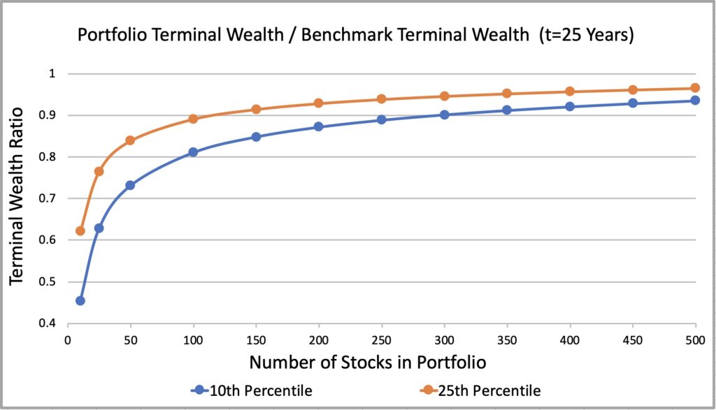
We can indirectly test our TWR formula for 10th and 25th percentile empirically by comparing theoretical predictions to empirical results from a study carried out by Chen & Israelov [5]. Chen & Israelov select equally weighted, randomly selected, monthly rebalanced portfolios from a population of 1000 biggest stocks in a 25-year period from 31-Dec-1994 through 31-Dec-2019. The authors calculate terminal wealth multiple (TWM) for 10th and 25th percentile (unlucky) outcomes and plot the curves as a function of number of stocks in portfolio. TWM is the terminal wealth (after 25 years) of the portfolio percentile divided by the starting capital. We can get from terminal wealth multiple to terminal wealth ratio by dividing TWM by the terminal wealth of the fully diversified benchmark portfolio.
We show the empirical result in the figure below and the theoretical prediction by our TWR formula in the next figure. We don’t know the exact idiosyncratic variance of a single stock in the empirical study, but we have estimated it for big stocks (about 1000 biggest stocks) from our Jan-1973 to Jun-2018 data and use this value in our theoretical prediction.
When we compare the empirical and theoretical figures below, we can see that the shape of the curves is almost identical and that the relative difference between the 10th and 25th percentile is very similar. Furthermore, Chen & Israelov mention that the terminal wealth multiple of the fully diversified benchmark portfolio is about 19. If we divide the TWM in the empirical figure by 19, we will get very close to TWR values shown in the theoretical prediction figure.
Overall, our TWR formula seems to predict the empirical outcome surprisingly accurately. Remarkably, our formula only takes one statistical parameter as an input: idiosyncratic variance of a single stock.

Further demonstrations of the diversification effect
We have derived equations and shown that they work empirically. Next, we will utilize the equations to further demonstrate how diversification effect works when we consider terminal wealth differences to fully diversified benchmark portfolio.
Portfolios are always equally weighted and randomly selected. The parameters of the benchmark are all equal to portfolio we examine except that the level of diversification (number of stocks) is different. E.g. in the figures where we examine the effect of leverage, benchmark is leveraged too.
Demonstrating terminal wealth ratio
In the figure below, we demonstrate portfolio’s median terminal wealth ratio for different portfolio sizes. Notice that TWR is now expressed as percentage difference to benchmark. Single stock portfolios typically lose close to 100% compared to benchmark terminal wealth in the long-run. Notice that this is not explained by the fact that most firms lose their value if we just wait long enough. This dismal result is achieved by randomly selecting the stock we invest in continuously (ignoring trading costs). Random selection is our baseline for the case where stock picking skill is not involved. Note that stock picking skill can be positive or negative (e.g. behavioural biases can be considered negative skill). One could argue that random selection is too optimistic assumption and investors in real life are more likely to possess negative than positive skill and are therefore likely to lose to randomly selected portfolio. Nevertheless, we consider randomly selected portfolio the best available baseline.
We can see from this figure also what was predicted by our equations: to keep terminal wealth ratio constant (to prevent it from decreasing), we need to increase diversification approximately in direct proportion to increase in time. It is easy to see e.g. that median TWR of a 1-stock portfolio at 10-year horizon is approximately equal (about -78%) to median TWR of 10-stock portfolio at 100-year horizon. Or that median TWR of a 10-stock portfolio at about 7.5-year horizon is approximately equal (-10%) to median TWR of 100-stock portfolio at about 75-year horizon.

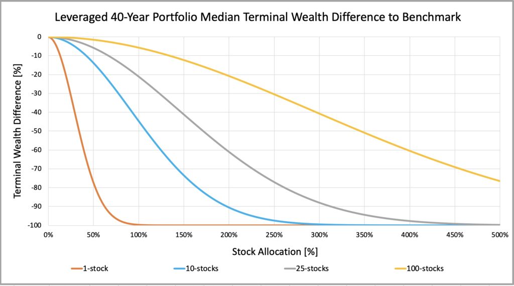
As mentioned, and demonstrated in the figure below, if there is one condition when diversification is beneficial, it is when your leverage is high. Measured as terminal wealth ratio, concentrated highly leveraged portfolio without some serious stock picking skill is suicidal.
Our TWR equation predicted that to keep TWR constant, we need to increase diversification approximately in squared proportion to increase in leverage multiplier. This is seen from the figure below: e.g. 25-stock portfolio has a TWR of about -20% at stock allocation 100% (leverage multiplier 1) while 100-stock portfolio (4 times more stocks) has the same TWR at 200% stock allocation (leverage multiplier 2). 2^2 = 4 times more stocks are required to keep TWR constant when stock allocation doubles from 100% to 200%.
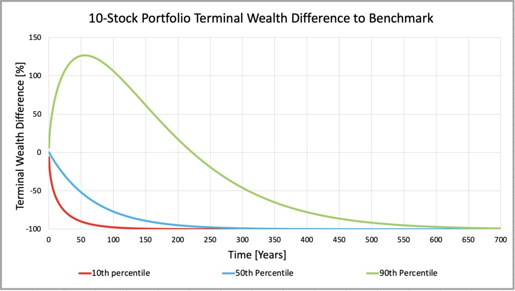
You may get lucky, but be aware that luck wears out over time. The figure below shows 80% confidence interval for 1-stock portfolio terminal wealth ratio. If you are lucky (the best 10% in the 90th percentile), you may beat your benchmark even after 20 years by sheer luck (variance). The next figure is almost identical, but is for 10-stock portfolio and has x-axis (time) multiplied by 10. Again, to keep terminal wealth ratio constant, you need to increase diversification approximately in a direct proportion to increase in time. With 10-stock portfolio the lucky ones may celebrate their benchmark beating returns even after 200 years of compounding.

Will 10 stocks make a diversified portfolio? At least we can tell from the figure below that it may depend on your time horizon and investing style. Without stock picking skill and measured as median TWR, less than perfectly diversified equally weighted portfolios of any size (any number of stocks) will approach 100% loss compared to their fully diversified benchmark as time approaches infinity. It is only a matter of time, but the process can be slowed down by diversification and e.g. by investing style selection. We can see that big stocks and high E/P value stocks require considerably less diversification compared to e.g. micro-cap stocks and low E/P growth stocks.

Demonstrating probability of losing to benchmark
Next, we further demonstrate the probability of losing to fully diversified benchmark.
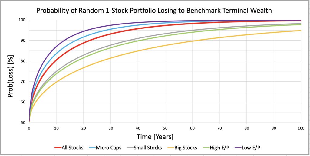
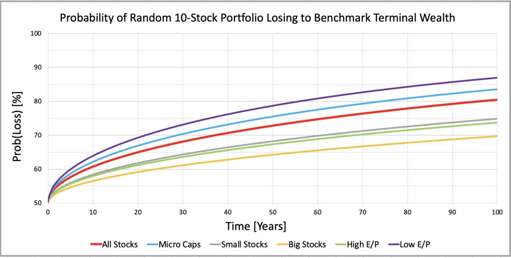
The figures below (for 1-stock and 10-stock portfolios) shows brutally how the probability of a randomly selected equally weighted portfolio losing to benchmark inevitably approaches 100% over time. We can affect how quickly the inevitable happens by diversification and by investment style selection. Again, we see that smaller stocks and e.g. growth stocks tend to lose to their benchmark quickly and require more diversification compared to e.g. big stocks and value stocks.
Similarly as with TWR, to keep the probability of losing to benchmark constant (to prevent is from increasing), we need to increase diversification approximately in direct proportion to increase in time horizon length. E.g. for all stocks, the probability of losing to benchmark with 1-stock portfolio is about 81% at 10-year horizon and the same 81% with 10-stock portfolio at 100-year horizon. In this respect, the importance of diversification increases as investment time horizon length increases.
If we multiply the time (x-axis) by ten, we can interpret the 1-stock portfolio figure as 10-stock portfolio figure with ten times longer time horizon. E.g. we can interpret that more than 95% of 10-stock portfolios – regardless the style we choose – will lose to their benchmark at 1000-year time horizon. It is only a matter of time.
In case you don’t want to wait to destroy your odds to beat the benchmark, there is a solution: use a lot of leverage and you don’t need that much time. E.g. using leverage multiplier 2, we only need (1^2)/(2^2) = 1/4 of the time to reach the same probability as with unlevered (leverage multiplier = 1) portfolio or (0.5^2)/(2^2) = 1/16 when compared to portfolio with leverage multiplier 0.5. We can again consider the question: will 10 stocks make a diversified portfolio? It may depend also on your allocation to stocks. The higher the allocation to stocks or leverage, the more likely the randomly selected equally weighted portfolio is to lose to its fully diversified benchmark.

Conclusions & Implications
Empirical relative terminal wealth difference between a randomly selected equally weighted less than perfectly diversified portfolio and its benchmark (terminal wealth ratio), as well as probability of losing to benchmark, can be modelled very accurately by mathematical models based on log-normal returns.
Theoretical relative terminal wealth difference to benchmark is a theoretical upper bound for empirical results implying that empirical results are typically slightly worse than predicted by the model. This is mainly because of fat-tailedness of individual stock returns.
Central limit theorem works very effectively for long-term randomly selected equally weighted portfolio’s involving only idiosyncratic variance, which makes theoretical model for predicting probability of losing to benchmark based on log-normal return assumption very precise empirically.
Despite the heterogeneity and the complexity of factors behind stock returns, portfolio’s relative terminal wealth difference to fully diversified benchmark and probability of losing to benchmark depend only on one statistical parameter: idiosyncratic variance of a single stock.
Conventional diversification analysis focuses on annualized standard deviation of arithmetic returns, but long-term investors eventually care about compound terminal wealth. When we focus on terminal wealth, we find that many conventional wisdoms concerning diversification no longer hold. Or that new aspects – absent from conventional diversification effect analysis – arise.
We find that, in the absence of stock picking skill, the importance of diversification increases as time horizon increases, that diversification becomes particularly important when allocation to stocks increases or when we leverage our portfolio and that importance of diversification depends on our selection of investing style.
To prevent our randomly selected equally weighted portfolio’s relative terminal wealth difference to fully diversified benchmark from decreasing and probability of losing to benchmark from increasing, we need to increase diversification in direct proportion to time and in squared proportion to leverage multiplier.
The importance of diversification is very much a function of selected investing style. E.g. small stocks, especially micro-caps, require more diversification compared to big stocks and growth stocks, classified based on E/P, require more diversification compared to value stocks.
In the long-run, randomly selected 1-stock portfolios lead to dismal terminal wealth compared to diversified benchmark and probability of losing to benchmark approaches one. The same happens to any less than perfectly diversified portfolio size, it just takes more time or leverage and this adverse development can be accelerated by selecting an investing style (benchmark) loaded with idiosyncratic variance.
References
[1] Kurtti, M. T. (2020). How many stocks make a diversified portfolio in a continuous-time world?
- 3.3.1 Derivation of diversification premium & diversification premium difference to benchmark
- 3.3.2 Estimation of diversification premium & compensation of differences in monthly number of stocks
- 4.1.1 Three distinct stock populations in the CRSP data
- 5.2.1 Empirical test for diversification premium difference to benchmark as a function of stock allocation
- 5.2.2 The effect of fat tails
- 5.6.1 Empirical test for the relationship between number of stocks and time horizon length
- 5.8 Investing style driving diversification effects
[2] https://en.wikipedia.org/wiki/Law_of_large_numbers
[3] https://en.wikipedia.org/wiki/Central_limit_theorem
[4] https://en.wikipedia.org/wiki/Log-normal_distribution
[5] Chen, Y. & Israelov, R. (2022). How Many Stocks Should You Own?
Article by Markku Kurtti