
We will see how the diversification assessment framework provided by conventional finance theory is not applicable to what long-term investors really care about – compounded returns. As long-term investors care about geometric (instead of arithmetic) expected return, we will find that diversifiable risk is not only uncompensated but costly. As a consequence, diversification is not only free, but negative price lunch. What are the implications of all this? Let’s have a look.
Arithmetic single period vs. Geometric compounded returns
The most famous phrase in finance is “diversification is the only free lunch” in investing by Harry Markowitz.
The phrase is true for annualized arithmetic returns for which diversification does not affect the mean (expected return), but reduces the risk (volatility i.e. standard deviation of returns around the mean). The lunch is considered free as by diversifying you don’t lose any expected return while you reduce your risk.
Annualized arithmetic returns are single period returns. Expected annualized arithmetic return is calculated as an expectation of an ensemble of single period returns. You can earn and enjoy annualized arithmetic returns in settings where you always invest the same amount of capital for each period and don’t reinvest the proceeds from period to next. Say that you play pool for $10 a game. You always invest the same $10 for each game and either double or lose your bet. If you have an edge (skill) you can enjoy arithmetic returns for your investment. But you can’t enjoy compounded returns and increase your wealth exponentially over time as you are not reinvesting your proceeds from one game to next. See Kelly’s story about arithmetic returns enjoying gambler financed by his wife with constant $1 weekly gambling allowance [1].
Most long-term investors want to grow their wealth exponentially over time. To be able to do that, investors need to reinvest their returns from one period to next. This happens automatically in the stock market where firms invest their proceeds to be able to make more in the future. We can think compounding as taking place continuously (this is not true exactly, but useful approximation). Firms may pay out dividends, which long-term compounder reinvests to keep his compounding process intact.
But there is a cost: if you want to enjoy the benefits of compounding, you need to pay volatility tax (also called variance drag). Variance drag means that your average annualized geometric (compounded) return is lower than your average annualized arithmetic (single period) return. Annualized volatilities of these two types of returns are approximately equal (when measured from returns with short enough time interval; like daily or monthly returns).
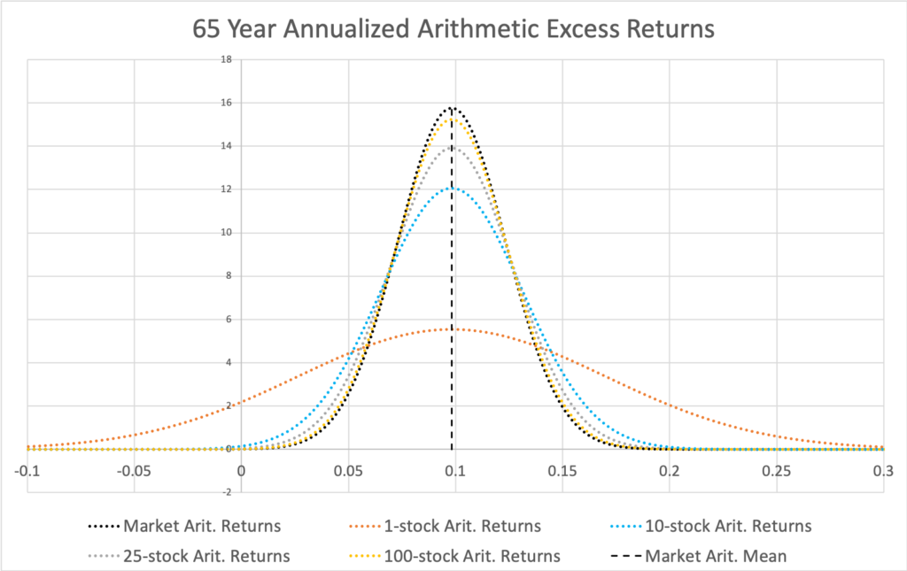
In the figure below, we see diversification as it is usually presented in the Markowitz framework using annualized arithmetic excess returns. Expected return is unchanged while more diversification decreases the volatility of the returns. The law of large numbers guarantees that the symmetric spread of returns converges towards the expected arithmetic excess return as depicted in the figure.
This figure, however, does not describe annualized returns of an investment which compounds over time i.e. an investment which reinvests its returns. Stocks are inherently such investments. With compounding, the law of large numbers applies to geometric, not arithmetic, returns. This means that with compounding over time (e.g. a stock portfolio with dividends reinvested), annualized return distribution converges towards geometric expected return and the symmetric (50% win, 50% lose) distribution of annualized arithmetic excess returns in the below figure does not exist. The distribution in the figure approximately exists for short-term constant starting capital single period stock returns (where the effect of compounding is minimal), such as stock purchases for a duration of one day with same dollar amount invested every trading day of the year. Compounding introduces skewness and will break the symmetry of the return distribution.
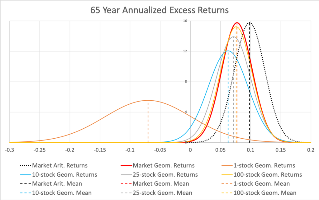
Investment over time in stocks is always subject to variance drag, meaning expected annualized geometric return (to which the law of large numbers now, with compounding, applies to) is lower than expected annualized arithmetic return. The effect of variance drag is shown in the figure below where the geometric mean excess return of a fully diversified portfolio is lower than arithmetic mean excess return (due to systematic variance drag) and the geometric mean excess returns of less than perfectly diversified portfolios are lower (due to idiosyncratic variance drag) compared to fully diversified portfolio.
The figure vividly demonstrates that idiosyncratic (firm specific, diversifiable) variance is not only uncompensated but costly. The cost is lower expected portfolio growth rate (geometric rate of return). Diversification, by lowering the cost, increases the expected annualized geometric return. Simultaneously (similarly as with arithmetic returns), diversification reduces risk (annualized standard deviation of geometric returns).
In other words, diversification is not only free but negative price lunch.
Geometric risk premium decomposed
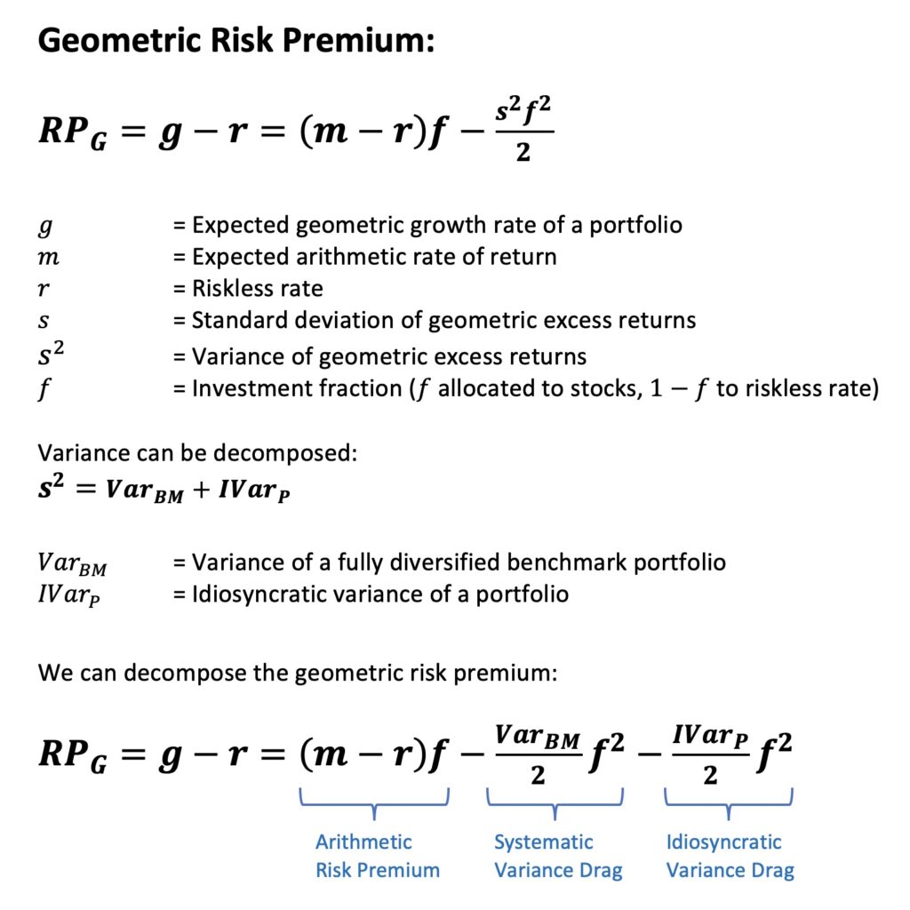
Geometric expected return and therefore also geometric risk premium (expected geometric return in excess of riskless rate) decreases as volatility increases. Below we first show the equation of geometric risk premium as it is usually presented (see Thorp [2] or my thesis [3]), then we decompose the equation to more intuitive form. Decomposed version demonstrates that geometric risk premium is arithmetic risk premium minus two variance drags: 1) systematic (undiversifiable) variance drag and 2) idiosyncratic (diversifiable, firm specific) variance drag. The latter drag explains why diversification, which decreases idiosyncratic variance, increases geometric risk premium.
It is worth noting that variance drag scales as a square of investment fraction emphasizing the importance of stock allocation and leverage. Diversification clearly is the more important the higher your stock allocation and especially if you leverage your stock exposure.
Note also that all of the formulas assume continuously compounded geometric returns (i.e. logarithmic returns: ln(1 + arithmetic return)). Also, all of the shown empirical results (like geometric risk premiums) use continuously compounded returns.
Details including derivations for most of the formulas and empirical results can be found from my thesis [3].
Sometimes you hear that diversification is important because there are some rare super stocks with very high long-term returns and missing those will cause you to lose to benchmark index. It is true that such super stocks exist, but the existence of super stocks is a consequence, not a cause. The mathematical root cause why super stocks exist is idiosyncratic variance. We can select our portfolio once and keep it unchanged (apart from rebalancing) for a long time or we can re-select our portfolio every month to randomize the super stock exposure over time, and the resulting return distributions will be very similar. Idiosyncratic variance causes both the existence of the super stocks and the total failures. By diversifying we mitigate idiosyncratic variance which is to say we mitigate the effect of both (losing and winning) tails of the return distribution. Simultaneously we increase our geometric expected return by mitigating idiosyncratic variance regardless of whether our portfolio includes super stocks or not.
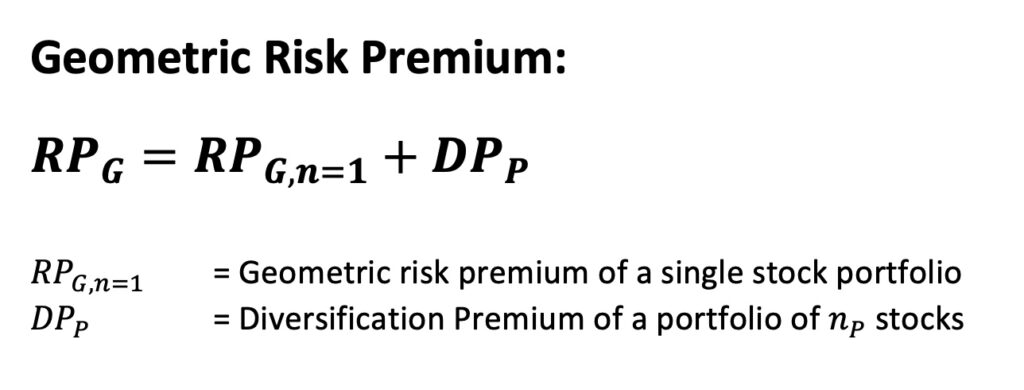
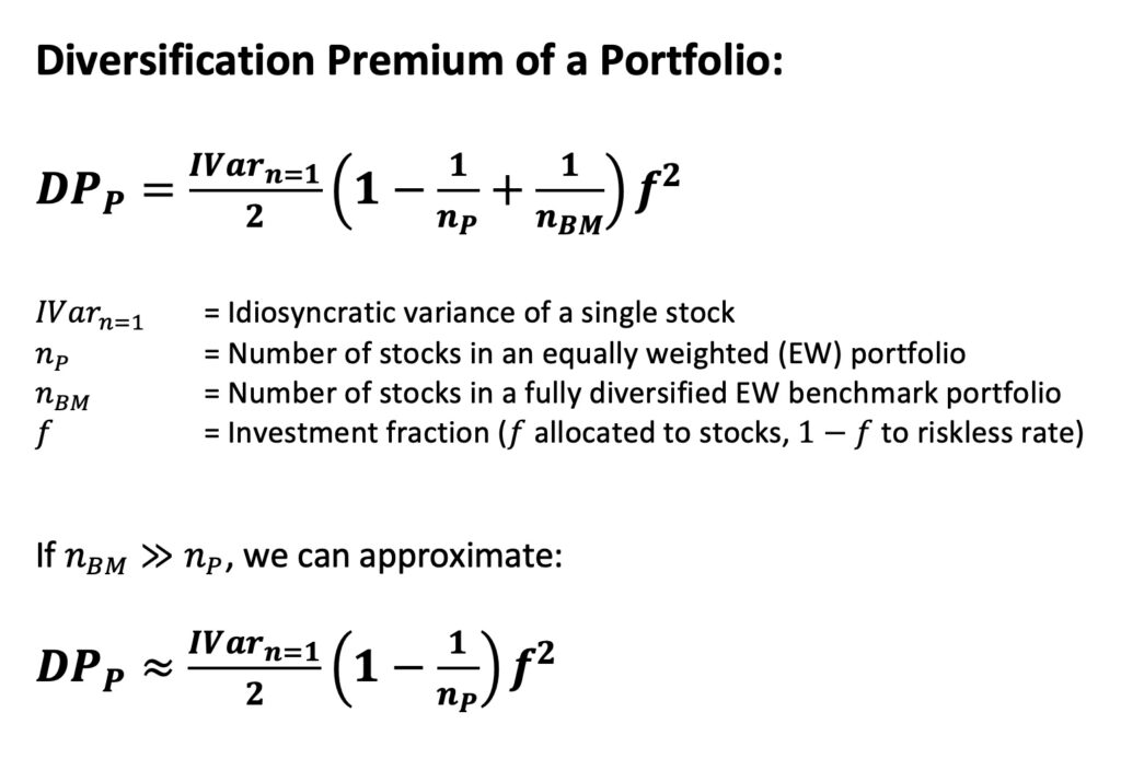
Another way to decompose geometric risk premium is shown below. We can define geometric risk premium as a sum of geometric risk premium of a single stock portfolio and diversification premium. Diversification premium is the increase in geometric risk premium (compared to single stock portfolio) attributable to diversification.
Diversification premium
Diversification premium is the difference between expected geometric growth rate of a portfolio and expected geometric growth rate of a single stock. Formula below shows how we can calculate diversification premium of an equally weighted portfolio. The key is the idiosyncratic variance of a single stock, which is scaled by the number of stocks (in portfolio and in benchmark portfolio) and investment fraction. The formula works when number of stocks in the portfolio is greater than one (if there is only one stock in the portfolio, there is no diversification and no diversification premium). Simpler approximate version of the formula can be used when the number of stocks in the benchmark is much higher than in the portfolio.
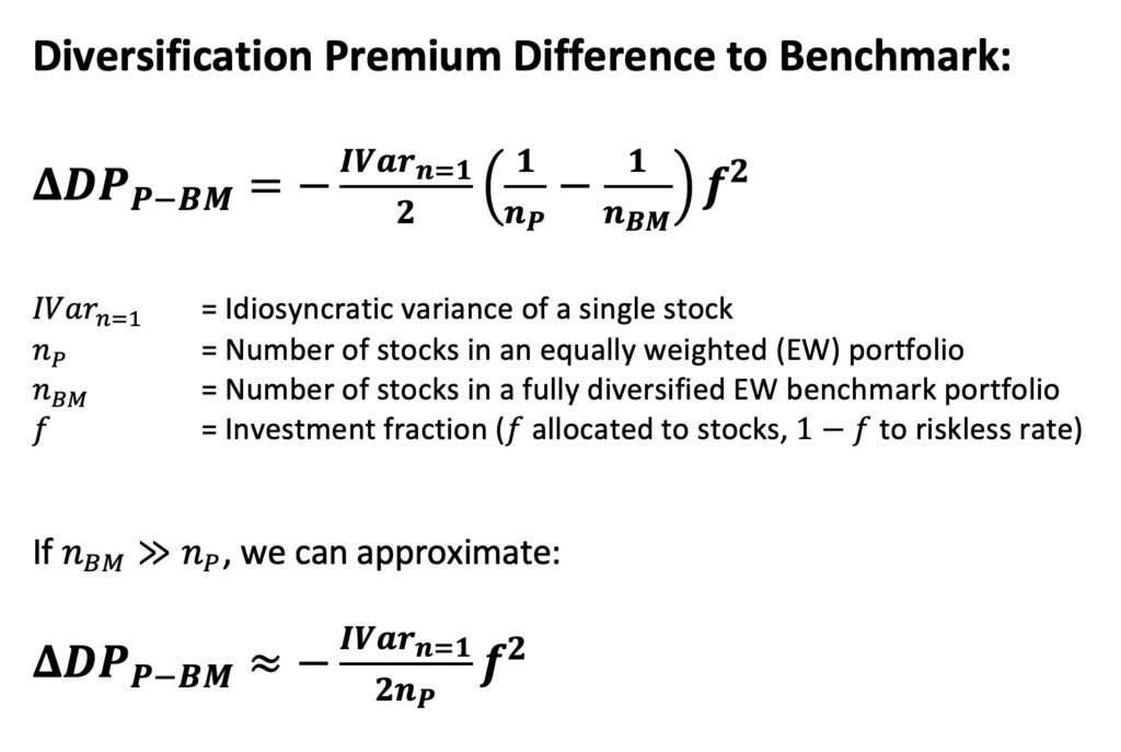
Diversification premium difference to benchmark
We can further define diversification premium difference to benchmark as the diversification premium difference between less than perfectly diversified portfolio and fully diversified benchmark portfolio. Diversification premium difference to benchmark is always negative (diversification premium of a less than perfectly portfolio is always lower than diversification premium of a fully diversified benchmark). The formula works when number of stocks in the portfolio is greater than one. If there is only one stock in the portfolio, then the approximate version of the formula must be used and it is exact.
Empirical geometric risk premiums as a function of diversification
We can test geometric risk premium and diversification premium as a function of diversification empirically. We use monthly CRSP data for all common stocks (delisting returns included) in the U.S. between Jan-1973 and Jun-2018. On average, we have 5472 stocks per month and most of the stocks are micro-caps. Results for all stocks are dominated by micro-caps and we therefore show results also for big stocks, small stocks and micro-caps separately. All portfolios are selected randomly (bootstrapping without replacement), equally weighted and rebalanced monthly. 50 000 randomly selected portfolios of each portfolio size are created in each empirical simulation. Single stock portfolios are exhaustive meaning all single stock portfolios are included instead of random selection. Benchmark portfolio includes all stocks in the tested category. We use monthly T-bills as riskless rate. Note that the empirical number of stocks vary from month to month. As we want to keep the weight of each month equal, we need to compensate for the differences in number of stocks. The method how to compensate the difference is given in [3]. Most of the figures and tables shown are from my thesis [3].
Realized returns are geometric returns. Empirical studies that use long-term realized (geometric) returns tend to find much larger number of stocks to be required for sufficient diversification compared to traditional studies focusing on annualized volatility. The theory of diversification premium and diversification premium difference to benchmark largely explain the results in these studies, like the famous Bessembinder study [4], using long-term geometric returns. Bessembinder found that single stock portfolios typically lose to monthly T-bill return and that less than perfectly diversified portfolios are likely to lose to fully diversified benchmark. Both results are visible in our empirical tests below.
Predicted theoretical values in the below empirical tests are derived using the approximate geometric risk premium formula below.
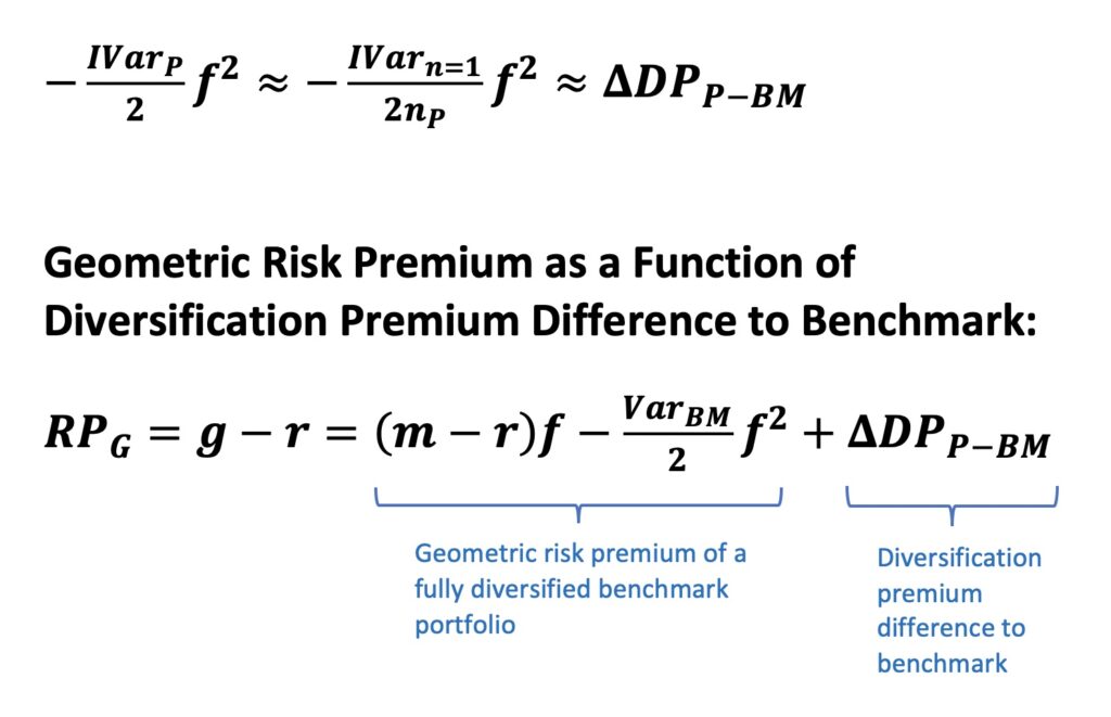
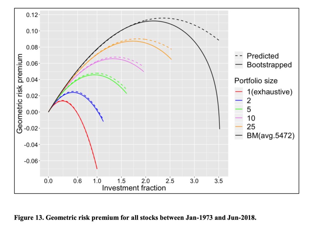
Figure below shows the result for empirical geometric risk premium test for all stocks. We can see that risk premium follows theoretical prediction accurately as long as investment fraction (leverage) is not too high. The shape of the curves is a parabola with a maximum, which is as expected for geometric risk premium (arithmetic risk premium is an infinitely rising line). The parabolic shape is in line with fractional Kelly criterion, which was described in my previous article The Kelly criterion, capital market parabola & the almighty Sharpe ratio.
The reason why empirical values are lower than theoretical predictions at high leverage is a combination of less than perfect rebalancing frequency (monthly) and fat tailed monthly return distributions. Theoretical formulas assume infinite rebalancing frequency. Simulation for each portfolio size is stopped when we find (for the first time) that a portfolio loses more than 100% of its equity during a month marking a ruin. Monthly rebalancing is too infrequent to prevent these occurrences from happening with leveraged portfolios.
We can see clearly that diversification is a negative price lunch and that idiosyncratic variance is costly. The diversification premium of a fully diversified benchmark portfolio is 14.8 percentage points at 100% stock allocation (Investment fraction = 1). It is clear that diversification becomes extremely important when portfolio is leveraged.
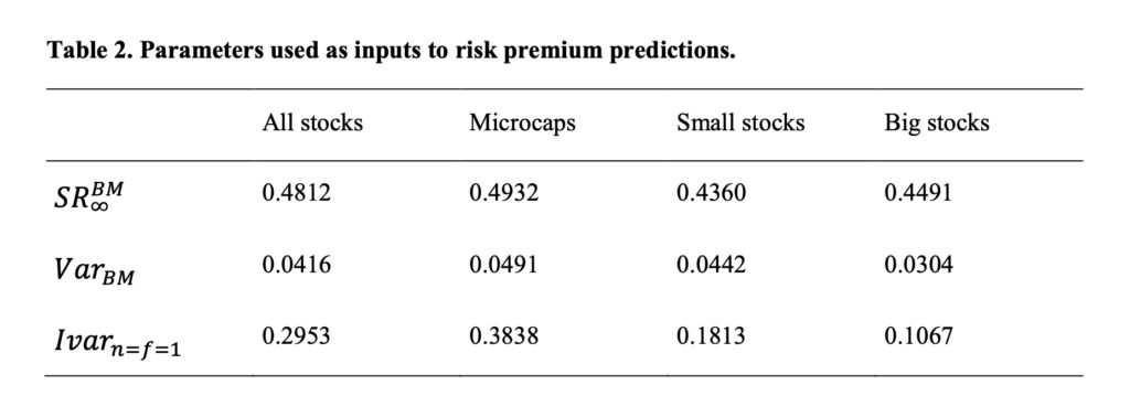
Previous figure was for all stocks. Let’s check the corresponding result also for micro-caps, small stocks and big stocks separately. Here are the empirical parameters.
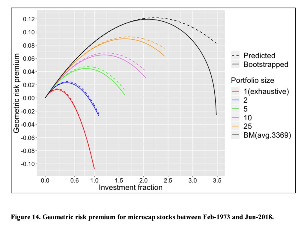
We see the result for micro-caps below. Results are even more extreme now that bigger stocks are excluded from the benchmark portfolio.
The same test for small stocks.
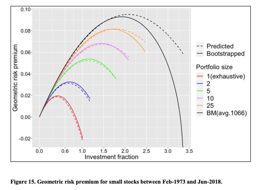
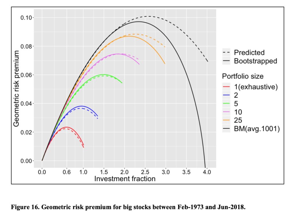
And the big stocks. With big stocks, single stock portfolio risk premium is barely positive at 100% stock allocation (more than 50% of big stocks win riskless rate). With small stocks and especially with micro-caps single stock portfolio risk premium is negative (more than 50% of small and micro-cap stocks lose to riskless rate).
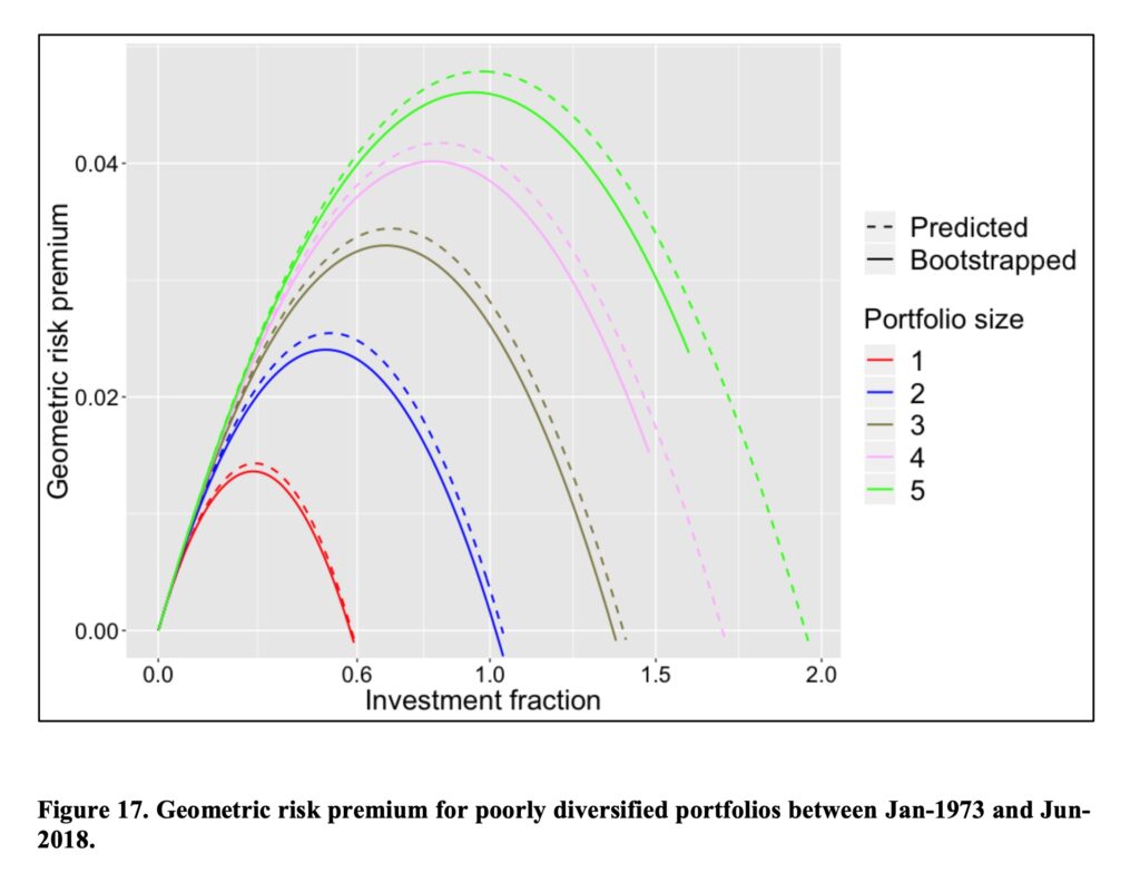
Let’s check the result for very poorly diversified portfolios among all stocks. We can see that 5 stock portfolios maximize their geometric risk premium at about 100% stock allocation. In other words, when your portfolio size is less than 5 stocks, you will increase your geometric expected return by lowering your stock allocation from 100% and investing the remaining part of your capital to T-bills. This may come as a surprise to many that you can increase your (geometric) expected return by taking less risk. Furthermore, we can see that with two stock portfolios, your geometric risk premium at 100% stock allocation is very close to zero i.e. the return of riskless rate (monthly T-bill). With single stock portfolios, you will by expectation lose to riskless rate.
Empirical diversification premium difference to benchmark
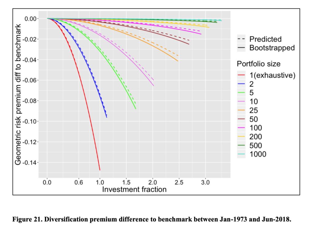
Diversification premium difference to benchmark is tested up to very large portfolios and we therefore use the accurate version of the formula for the theoretical prediction. Prediction is very accurate until we go further into leveraged portfolios. Monthly rebalancing is not enough for leveraged portfolios with fat tailed returns. We tested (not shown here, see [3]) cutting off one permille from both tails (0.1 & 99.9 percentile monthly returns) and the prediction became extremely accurate also with higher leverage.
We can see from the below figure how diversification increases expected geometric return and how the investment fraction and leverage make diversification increasingly important. With high enough leverage, even hundreds of stocks still lose noticeably to fully diversified benchmark. We are not considering the risk reducing aspect of diversification at all, but even by only considering expected return differences (an aspect which does not even exists in conventional finance theory), it is very difficult to come to conclusion that ten stocks are enough. With considerable leverage, it is difficult to come to conclusion that less than 50 stocks would be anywhere near sufficient. To demonstrate the effect of leverage, consider that 10 stock portfolio loses on average about 1.5 percentage points to benchmark at 100% stock allocation, but about 2^2*1.5 = 6 percentage points at 200% stock allocation. Fat-tailedness of stocks returns further increase the need for diversification.
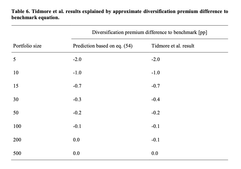
In addition to our own empirical study, we can use Tidmore et al. study [5] as an independent empirical study to test our theoretical diversification premium difference to benchmark formula. We can see that our formula predicts the diversification premium difference to benchmark very accurately.
Realized returns are geometric returns and long-term investors almost exclusively measure and care about geometric returns. Risk premium can be measured either by using arithmetic or geometric returns. One of the best references for historical risk premiums across countries is the yearly report by Dimson, Marsh & Staunton [6], which uses geometric risk premium.
If we assume that investors care about geometric risk premium, then – all else equal – we should assume higher market valuations and lower forward-looking risk premium compared to history. Let’s see why.
We can approximate (at 100% stock allocation) the loss to fully diversified benchmark (diversification premium difference to benchmark) simply by dividing half of single stock idiosyncratic variance by the number of stocks. Using empirical idiosyncratic variances, the loss for 5 stock portfolios is roughly 1, 2 & 4 percentage points for big, small & micro-cap stocks, respectively. Or 0.5, 1 & 2 percentage points for 10 stock portfolios.
Back in the day, before cheap index funds and ETFs, trading costs and other frictions were high and the marginal benefit of diversification diminished quickly. We can imagine 5 or 10 stock portfolios to have been much more reasonable and common than portfolios containing hundreds of stocks.
Given the small portfolio sizes with large diversification premium difference to benchmark, rational investors should have required compensation for their idiosyncratic variance drag implying lower valuations and higher required risk premium (measured at diversified index level). Today, with the availability of modern financial technology allowing practically free full diversification, investors don’t need to bear idiosyncratic variance and have no need to require as high risk premium what we have seen historically. Not accounting for risk differences, we should assume historical and forward-looking required geometric risk premiums to be equal after accounting for idiosyncratic variance drag, trading costs and other frictions. Following this logic, the baseline (not accounting for risk reduction via better diversification) for today’s forward-looking required geometric risk premium should be historical required geometric risk premium minus historical idiosyncratic variance drag, trading costs and other frictions. Similarly, we should assume forward-looking size premium to be materially lower compared to history as small stocks, and especially micro-caps, are loaded with idiosyncratic variance.
This line of thinking was introduced to me by pseudonym Jesse Livermore [7]. Jesse Livermore justified lower forward-looking risk premium by lower risk thanks to today’s practically free diversification. Our analysis focuses on increased geometric expected return as a function of increased diversification. Reduced risk comes on top of increased expected return, further strengthening our case for lower required forward-looking risk premium.
Empirical diversification premium as a function of firm size and investment style
Idiosyncratic variance is the key characteristic which determines how beneficial diversification is. We have shown how we can derive the interesting metrics from the idiosyncratic variance of a single stock.
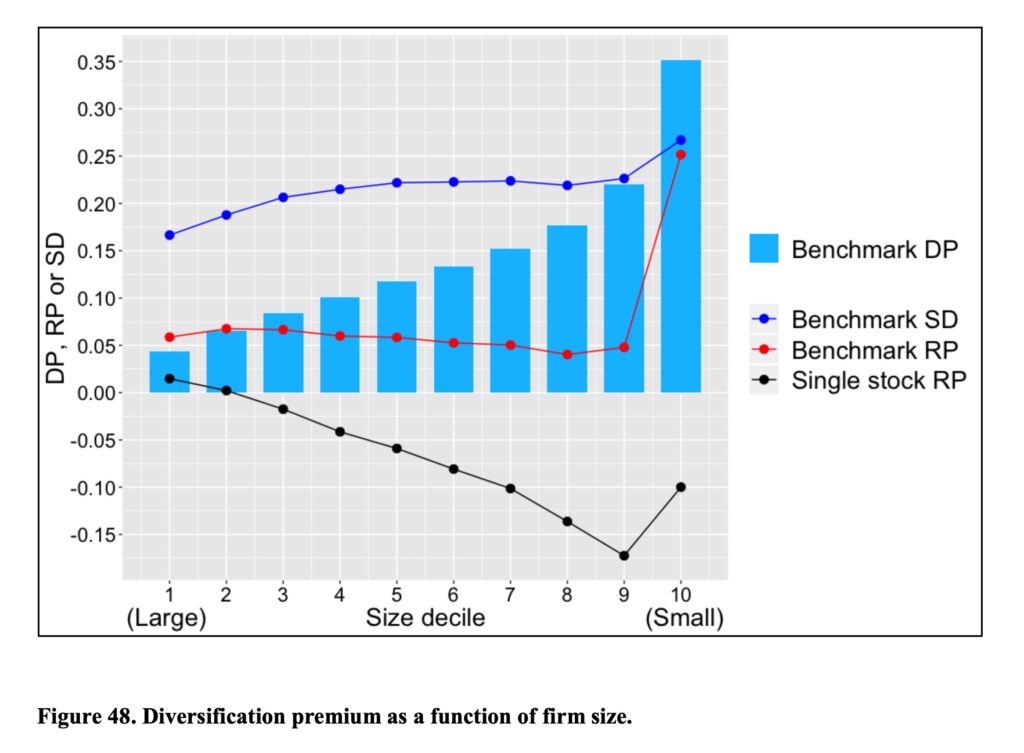
We can create different benchmark portfolios and measure the idiosyncratic variance of a single stock within the selected benchmark. For example, we can create size deciles based on market capitalization. We can see from the below figure that benchmark diversification premium (the difference in geometric risk premium between fully diversified benchmark and single stock portfolio) is monotonically increasing as we move from biggest to smallest decile. Diversification becomes extremely important when we consider the smallest decile of stocks.
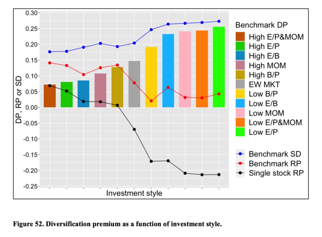
We can sort stocks also based on investing styles. Combined high earnings yield & high momentum style benefits the least (requires the least) from diversification while low earnings yield style requires (benefits) the most diversification. Interestingly, the styles which have had high returns historically seem to have required the least diversification. Potential explanation could be investor’s lottery preferences meaning that many investors prefer and pay higher price (implying lower returns) for stocks which may pay off big. Those stocks are the ones with high idiosyncratic variance (high diversification premium).
Also, we can see positive correlation between systematic style volatility (“Benchmark SD”) and diversification premium (which is effectively idiosyncratic variance i.e. idiosyncratic volatility). The styles (and the same applies to size deciles) with the lowest systematic volatility have had the lowest diversification premiums (idiosyncratic volatility).
Diversification premium as a function of market regimes
Contrary to conventional wisdom, diversification benefit is typically higher in bear markets. Diversification was very beneficial both in tech bubble burst and in the global financial crisis. The thing is that diversification eliminates idiosyncratic volatility and idiosyncratic volatility typically peaks when systematic volatility peaks i.e. in bear markets.
We can see in the animation below how the previous cycle winners are violently shaken off by the market during the tech bubble and its bursts and during the global financial crisis. More technically, idiosyncratic variance rises dramatically as the market experiences brutal, regime changing, bear market. Idiosyncratic variance is calculated for each month and annualized. Diversification premium (the difference between expected growth rate of a portfolio and expected growth rate of a single stock) of an equally weighted (EW) benchmark index ranges between 6.0% and 60.4% and is on average 14.8% per annum. Idiosyncratic growth rate (g) = growth rate of an individual stock – growth rate of an EW benchmark index.
Consistency of diversification premium over time
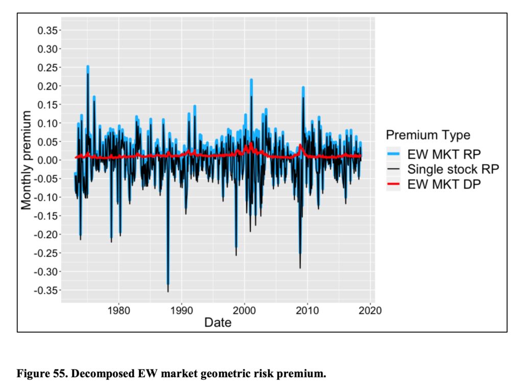
Earlier we saw how to decompose geometric risk premium to single stock risk premium and diversification premium. In the figure below, we see the geometric risk premium of an equally weighted market (blue) and its determinants: geometric risk premium of a single stock portfolio (black) and diversification premium (red) as a function of time. These are monthly premiums (not annualized).
We can see with bare eye that single stock risk premium volatility is to blame for the market volatility. The blue curve is black and red added together. The blue parts reaching above black are attributable to diversification premium. The difference may not look like much, but try compounding the difference first to yearly values, then to decade and so on.
Like we saw in the animation and now in this figure, diversification premium is always there and often raising its head when needed the most. Unlike the very volatile single stock risk premium and market risk premium, diversification premium is always positive and consistent over time.
Conclusions & Implications
Markowitz single period model based on annualized arithmetic returns can’t be used to assess the diversification effect on returns compounded over time. The Markowitz diversification effect (risk reduction) on standard deviation is (practically) the same as with compounded returns, but the effect on expected return is completely different.
When considering returns compounded over time – like ~100% of long-term investors do – idiosyncratic variance is not uncompensated but costly and diversification comes with an expected geometric return premium. Diversification is not free but negative price lunch.
The conventional way to estimate forward looking expected geometric returns by extrapolating realized long-term market return without taking diversification premium differences into account is simply wrong.
Diversification premium is determined by portfolio’s idiosyncratic variance, which is scaled by the square of investment fraction (stock allocation). High stock allocation emphasizes diversification premium. Leveraging makes diversification extremely important.
Diversification premium difference to benchmark (idiosyncratic variance drag) compounds over time. Given enough time, even the slightest diversification premium difference to benchmark can cause a big difference in typical terminal wealth.
Mitigating idiosyncratic variance via diversification is enough. We don’t need to care or worry about finding ten baggers or the winner takes it all stocks. One example of not necessarily needing the super stocks to have good outcomes is high earnings yield (value stocks selected based on low P/E) stocks, which are not likely to include super stocks (they have very low idiosyncratic variance), but have performed handsomely in the past.
Fat-tailedness of stock returns futher increase the need for diversification.
Small/micro-caps may be more inefficiently priced, but the flip side is that they come with much higher idiosyncratic variance i.e. much higher variance drag. There is no free lunch in harvesting returns in less efficiently priced pool of smaller firms as you need more stock picking skill diluting diversification to overcome the idiosyncratic variance disadvantage compared to big stocks.
Style matters. Styles with high historical returns typically require much less diversification (have lower idiosyncratic variance) compared to opposite styles. E.g. high E/P style reflects style returns already with small portfolio sizes while low E/P style is much more about firm specific factors. One could argue that high E/P style stock pickers, even with relatively concentrated portfolios, may not have much pure stock picking skill but have an exposure to profitable style.
Conventional wisdom has it that diversification does not help when it is the most needed because correlations rise and systematic volatility peaks at crisis. But diversification was never supposed to help mitigate systematic variance. If it did, we would not have risk premium. We diversify to reduce idiosyncratic variance and, based on history, idiosyncratic variance (diversification benefit) is at its highest during severe bear markets.
We can decompose geometric risk premium to geometric risk premium of a single stock and diversification premium. Geometric risk premium of a single stock explains market volatility. Unlike geometric risk premium, diversification premium is always positive and, compared to risk premium, very consistent over time.
Historical geometric equity risk premium before modern financial technology is a highly theoretical construct which was never practically achievable to investors. (Same applies to size premium). If we deduct the historical idiosyncratic variance drag, trading costs and other frictions from the historical risk premium (or size premium) and account for reduced risk, we end up with a much smaller number. This is one piece to equity risk premium puzzle.
References
[1] Kelly, J. L. (1956). A New Interpretation of Information Rate
[2] Thorp, E. O. (2006). The Kelly criterion in blackjack, sports betting and the stock market
- For geometric risk premium (or expected geometric growth rate to be exact), see derivation of eq. 7.2
[3] Kurtti, M. T. (2020). How many stocks make a diversified portfolio in a continuous-time world?
- 3.2 Derivation of geometric risk premium
- 3.3.1 Derivation of diversification premium & diversification premium difference to benchmark
- 3.3.2 Estimation of diversification premium & compensation of differences in monthly number of stocks
- 3.3.8 Decomposing risk premium
- 5.1.1 Empirical geometric risk premium
- 5.2.1 Empirical diversification premium difference to benchmark & Tidmore et al. study result analysis
- 5.2.2 The effect of fat tails
- 5.8.1 The effect of firm size
- 5.8.2 The effect of investing style
- 5.9 The consistency of historical geometric risk premium
[4] Bessembinder, H. (2018). Do stocks outperform treasury bills?
[5] Tidmore, C., Kinniry, F. M., Renzi-Ricci, G. & Cilla, E. (2019). How to increase the odds of owning the few stocks that drive returns
[6] Dimson, E., Marsh, P. & Staunton, M. (2022). Credit Suisse Global Investment Returns Yearbook 2022 Summary Edition
[7] Jesse Livermore (2017) Diversification, Adaptation, and Stock Market Valuation
Article by Markku Kurtti
Pingback: Isyysblogi: Win, win ja vielä kerran win – Isyysvapaa
Pingback: Helmikuu 2024 – Perheenlisäystä – Isyysvapaa
An excellent article. It is unfortunately true that most leading finance textbooks ignore or are not aware of the major difference between arithmetic and geometric mean. And this is not just some trivial academic point, it strongly impacts individual investors. Although ergodicity has recently become popular in economics.
It is a long article that might be better presented in two separate parts, an introduction and then deeper analysis.
I have a few trivial points i noted as i read the article:
It would be easier if this entirely took the viewpoint of historical returns. Discussing expected returns requires specialized notation but it also implies assumptions about market efficiency and investor behaviour that complicate things.
In a simple introduction it would be easier to assume an investment fraction of 1 and write the equations on that basis. This means that we are focusiing on the impact of diversification on share portfolios.
Figure 13 is very important and above this is written: The diversification premium of a fully diversified benchmark portfolio is 14.8 percentage points at 100% stock allocation (Investment fraction = 1). However it appears from the figure that the premium is 0.08.
It would be clearer if the charts just noted a percentage return rather than a decimal.
It is a common feature of academic articles that portfolios are rebalanced monthly. But in the real world this never happens because of transaction costs. So i would have preferred the simulations to be annual to make them more useful.
Essentially I would welcome a table in the conclusion that shows the return and Sharpe ratio of the benchmark compared to portfolio sizes that range from 10 to 100 using annual rebalancing. This very easily shows the reader the benefit of diversification.
Thank you again for a brilliant piece of work that investors should be aware of.
Dr Graham Buckingham
Thank you, it think these are good comments.
I agree yearly rebalancing would be more realistic considering real portfolios retail investors have. I have been thinking about doing some tests and writing a post about the effect of different rebalancing frequencies.
Regarding diversification premium in figure 13. I define diversification premium as “the difference between expected geometric growth rate of a portfolio and expected geometric growth rate of a single stock”. This difference is close to 15 percentage points when we calculate the difference between the fully diversified portfolio and single stock portfolio. Geometric risk premium for the fully diversified portfolio (difference to riskless rate) is about 8%.
Really instructive and superb structure of content material, now that’s user genial (:.