
Consider a clairvoyant who can accurately predict two market parameters, Sharpe ratio and volatility, for the forthcoming 10-year period. Clairvoyant selects his stock allocation (leverage multiplier) based on these two parameters, rebalances back to target leverage monthly and holds his selected stock allocation for the 10-year period. The cost of leverage is equal to riskless rate and our clairvoyant is immune to margin calls.
There is a plenty we can learn just by observing how the clairvoyant chooses his leverage multiplier to time the market and how he performs against a static 100% stock allocation.
As most of us are not clairvoyants, we need to estimate our future parameters. We will see that it is not only the estimated expected return, but also the estimated volatility that should be considered when determining leverage multiplier.
The math behind clairvoyant’s decisions
In my earlier article The Kelly criterion, capital market parabola & the almighty Sharpe ratio, we showed that expected excess growth rate maximizing leverage multiplier, full Kelly allocation, is determined by dividing portfolio’s Sharpe ratio by portfolio’s volatility (f* = SR/s). We also showed that maximum expected excess growth rate (growth rate in excess of riskless rate, g – rf) of a portfolio, compounding process capacity, is determined as one half of portfolio’s squared Sharpe ratio: max(g – rf) = SR^2/2.
Notice that our Kelly formula for maximum expected excess growth rate at full Kelly allocation gives its output as continuously compounded excess growth rate (g – rf). Our clairvoyant prefers his returns in more commonly used yearly compounded CAGR format, which is found by first compounding continuously compounded excess growth rate for one year: excess CAGR = exp(g – rf) – 1. Finally, clairvoyant adds riskless rate to his excess CAGR and arrives to formula: CAGR = exp(g – rf) + rf – 1. By substituting compounding process capacity, we find CAGR capacity: max(CAGR) = exp(SR^2/2) + rf – 1.
CAGR maximizing leverage multiplier
It may come as a surprise to many that optimal strategy for risk neutral compounder, an investor who ignores risk and only cares about maximizing compound return, is simply: 1) maximize the Sharpe ratio of the portfolio and 2) leverage until volatility equals Sharpe ratio. In other words, an investor who only cares about maximizing the expected growth rate of his portfolio only needs to care about two parameters: Sharpe ratio and volatility. If portfolio’s volatility exceeds portfolio’s Sharpe ratio, expected growth rate starts to decrease. So even if risk neutral compounder does not care about risk per se, he better care about limiting his volatility to the level of his Sharpe ratio.
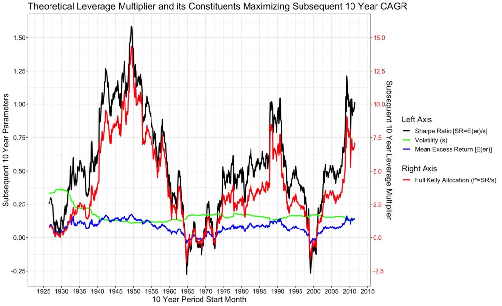
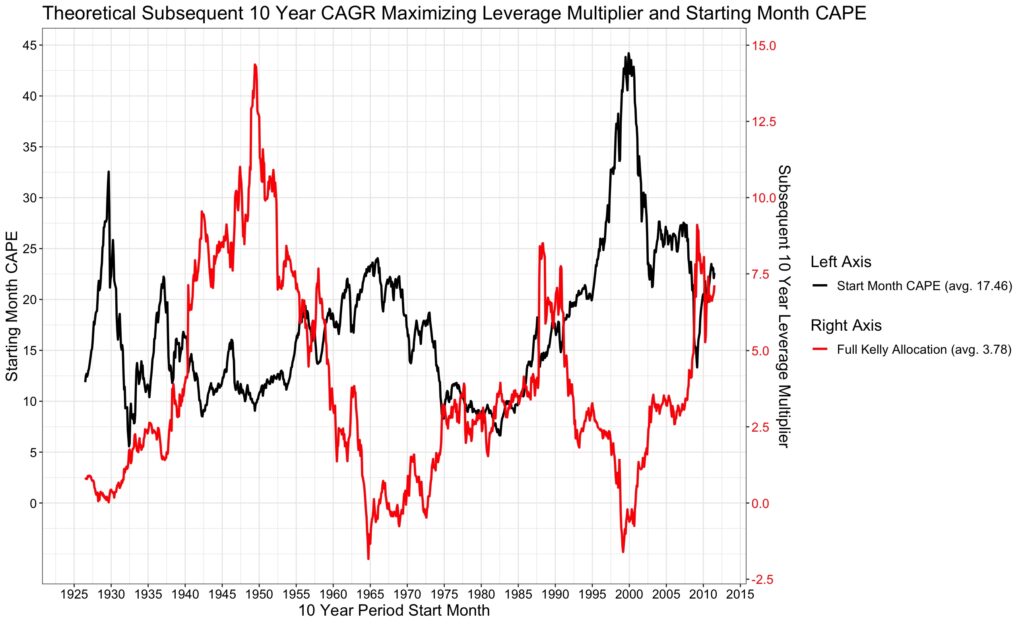
Sharpe ratio contains both expected arithmetic excess return (numerator) and volatility of the excess returns (denominator). Figure below shows all of the constituents of CAGR maximizing full Kelly leverage and the actual full Kelly leverage multiplier selected by the clairvoyant in rolling 10-year periods.
Leverage multiplier varies wildly between the minimum of -1.83 (Oct/1964) and the maximum of 14.36 (Jun/1949).
Our data is monthly U.S. market data from Kenneth French data library [1] between Jul-1926 and Jun-2021.
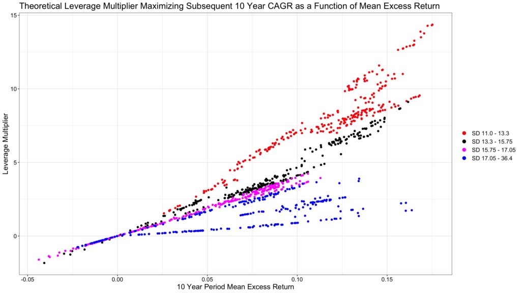
CAGR maximizing leverage multiplier must be a function of arithmetic mean excess return of the period, right? Yes, the figure below shows that if your mean excess return is low, your leverage multiplier is always low and even negative (meaning we are shorting the market) when mean excess return is negative. But at medium to high mean excess returns, the shape is not a line but more like a fan. Why a fan?
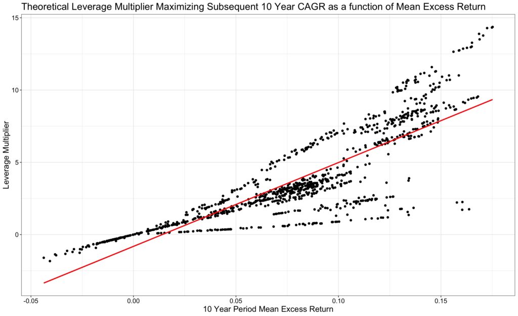
It is a fan because of different volatility regimes between the periods. CAGR maximizing leverage multiplier is at its highest value when expected excess return is at highest and volatility is in its lowest quartile. Regardless of the expected excess return, leverage multiplier never achieves very high values if volatility is above median volatility among all periods. Volatility of volatility (variability of volatility between periods) clearly is a risk to consider when leveraging a portfolio.
CAGR capacity
CAGR capacity is the maximum achievable CAGR, which is achieved at full Kelly leverage. The figure below shows CAGR capacity as a function of mean excess return. Again, we see that maximum CAGR is a function of expected return, but also a function of volatility. Super high CAGR can only be achieved when volatility is below median. High mean excess return can lead to very high, but also to low CAGR capacity.
In my earlier article The Kelly criterion, capital market parabola & the almighty Sharpe ratio we showed that increasing CAGR capacity (maximum CAGR) expands risk adjusted CAGR opportunity set available to investor. Kelly leverage and CAGR capacity therefore are informative to stock allocation decisions in general, not only to extreme case of optimal leverage leading to maximum CAGR. CAGR capacity is important for risk averse compounders too, because when CAGR capacity is high, the opportunity set available to risk averse compounders (utilizing lower than full Kelly leverage) is large and offers high risk adjusted returns.

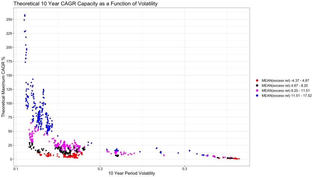
Next figure presents CAGR capacity as a function of volatility. Annualized maximum CAGR has exceeded 25% only when annualized 10-year period volatility has been below 20% and when mean excess return has been above (or close to) its median. 50% maximum CAGR has been exceeded only when volatility has been below 15% and when mean excess return has been in (or close to) its highest quartile.
At the end of the day, both expected excess return and volatility matter, but it is Sharpe ratio (or one half of square of Sharpe ratio to be more exact) that determines CAGR capacity. The figure below shows that maximum CAGR is dictated by Sharpe ratio and small deviations from the curve are due to differences in riskless rates between different periods. It is clear from the figure that high Sharpe ratio is very difficult to achieve if volatility is high. In general, to increase Sharpe ratio, it is much easier to mitigate the volatility of the portfolio by increasing diversification than to increase portfolio’s expected return.
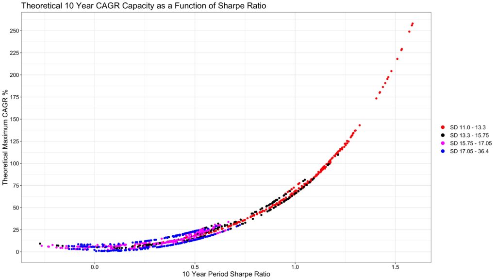
Market timing clairvoyant vs. static 100% stock allocator
How well the clairvoyant has done compared to static 100% static allocation? In the figure below, we see rolling 10-year periods (start date adjusted with monthly step size) between Jul-1926 and Jun-2021. For each 10-year period, we plot realized CAGR and realized maximum drawdown from starting capital for static 100% allocation and for clairvoyant’s CAGR maximizing full Kelly leverage (f* = SR/s). In addition, we plot theoretical predicted maximum clairvoyant CAGR (based on max(CAGR) = exp(SR^2/2) + rf – 1).
Note that monthly return data downplays drawdowns. Had we used daily data, drawdowns would have been noticeably worse. In addition to monthly data, riskless return provides some cushion against drawdowns especially in periods when riskless rate has been high.
As expected, the figure below tells us that clairvoyant beats the static 100% stock allocation investor. Average CAGR of the fully Kelly clairvoyant is 22.2% while 100% static allocation achieves 10.4%. But there is a cost in form of much higher maximum drawdowns. Clairvoyant’s average maximum drawdown is 33.9% compared to 16.2% for the static 100% allocation. Clairvoyant has many periods with close to 100% drawdown and 25 periods where equity is lost and clairvoyant is ruined. Note that periods where clairvoyant is wiped out are counted as -100% CAGR and drawdown meaning that we have forgiven clairvoyant’s debt after ruin.
But how can a clairvoyant using the Kelly criterion be ruined, shouldn’t that be impossible? Yes, it is impossible for clairvoyant Kelly investor to be ruined if all assumptions for Kelly criterion are fulfilled. Assumptions include continuous returns and rebalancing to target allocation at infinite frequency. Our clairvoyant is lazy and rebalances monthly. The higher the leverage, the more frequently we need to rebalance to target allocation. E.g. if we have 10x leverage, -10% month is enough to wipe us out with monthly rebalancing. With daily rebalancing, -10% day, which is not unheard of either, is enough to wipe us out. Markets are not always open and prices can have quick jumps meaning returns are not continuous. In practice, it is not possible to exclude the possibility of ruin no matter how frequently we rebalance. When leverage is high, tail protection becomes of vital importance.
Thanks to too low rebalancing frequency and non-continuous returns, clairvoyant is on average clearly behind theoretical predicted average CAGR of 31.8%. We can conclude that if full Kelly investing is this risky for a clairvoyant who can foresee relevant market parameters, it certainly is extremely risky to us mere mortals who need to estimate those parameters.
For comparison, theoretical full Kelly leverage multiplier for whole 95-year period is 2.40 and theoretical CAGR capacity is 14.0%. Corresponding average values for rolling 10-year periods are 3.78 and 31.8%. Clearly the shorter period a clairvoyant can predict the better positioned he is to monetize his gift.

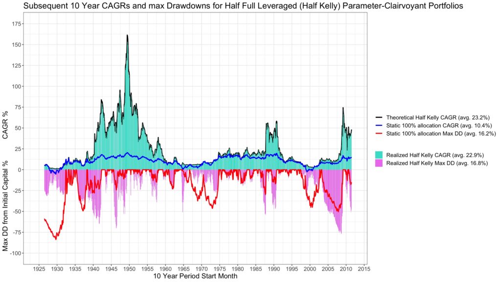
How about a half-Kelly investor, who invests half of full Kelly allocation?
We showed in my earlier article Drawdown risk = portfolio volatility normalized by Sharpe ratio that, excluding the effect of return time series autocorrelation, expected drawdown is determined by fraction of full Kelly allocation. Keeping fraction of full Kelly allocation constant means that drawdown risk (expected drawdown) is kept constant.
Half-Kelly portfolio is expected to have about half of the maximum drawdown from starting capital of full Kelly portfolio. This seems to be the case here as half-Kelly clairvoyant has an average of 16.8% maximum drawdown from starting capital compared to 33.9% for full Kelly clairvoyant. Risk is halved.
While risk is halved, theoretical average CAGR is about 3/4 (would be exactly 3/4 had we expressed growth rate in continuously compounded format) of full Kelly CAGR. Now, with half-Kelly, realized average CAGR is practically equal to theoretical predicted average CAGR. Realized half-Kelly CAGR at 22.9% is actually higher than realized full Kelly CAGR at 22.2%. Monthly rebalancing frequency is now sufficient and there is not a single period where half-Kelly clairvoyant is wiped out or has significantly lower CAGR than predicted by the theory.
We can find the fraction of full Kelly allocation for which stock allocation is on average 100%. This occurs at 0.265 times full Kelly allocation. Using 0.265-Kelly allocation, we can test what is the benefit (compared to static 100% allocation) of market timing with perfect 10-year foresight.
Figure below shows that clairvoyant with 0.265-Kelly allocation beats static 100% allocator both measured by average CAGR (14.6% vs. 10.4%) and average maximum drawdown (9.0% vs. 16.2%). Risk adjusted return (Avg. CAGR)/(avg. max drawdown) is about 2.5 times higher for clairvoyant. Clairvoyant demonstrates that there is potential in market timing, especially to boost risk adjusted return. To realize the potential without the gift of foreseeing the future parameters, of course, is not an easy task.

Market timing based on Shiller CAPE
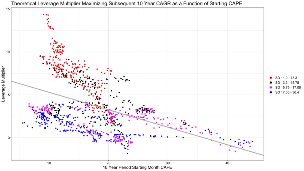
Shiller CAPE, along with other valuation metrics, is shown to have some predictive power on long-term stock returns. And many base their market timing decisions on market valuation metrics like Shiller CAPE. The figure below seems to support using Shiller CAPE for market timing. Highest optimal leverage multipliers have been achieved when CAPE has been relatively low (market has been cheap).
But in closer examination, it is the fan shape again. Optimal leverage for the forthcoming 10-year period has never been high when CAPE has been high. But CAPE seems to lose a lot of its predictive power when the market gets cheaper. When CAPE has been below 10, the range for optimal, CAGR maximizing, leverage multiplier has been huge. Clearly CAPE, or any valuation metric, alone is insufficient to determine leverage multiplier. Volatility and, even more importantly, volatility of volatility needs to be mitigated and/or predicted to make market timing by adjusting stock allocation more robust. On the other hand, successful mitigation of volatility and volatility of volatility, e.g. by diversifying across asset classes and strategies, may reduce the benefits of market timing.
What have we learned from the clairvoyant?
We have learned that risk neutral compounder, an investor who only cares about maximizing the expected growth rate of his portfolio, needs to care about only two parameters: Sharpe ratio and volatility. Contrary to common belief, market timing (leverage multiplier selection) should not be based on expected return alone, but risk adjusted return (Sharpe ratio) and risk (volatility).
Historical range for theoretical optimal, CAGR maximizing, leverage multiplier for a 10-year period has been huge. Lowest optimal leverage has been -1.83 and highest 14.36.
Theoretical optimal, CAGR maximizing, full Kelly leverage multiplier (and therefore the range of leverage multipliers to choose from) can be very high only if both expected excess return is high and volatility is low.
CAGR capacity, the highest achievable leveraged CAGR, (and therefore the range of returns available to risk averse compounder) can be very high only if both expected excess return is high and volatility is low. CAGR capacity is determined by the (one half of square of) Sharpe ratio of the portfolio.
Historically, very high Sharpe ratio, and therefore very high CAGR capacity, has been impossible to achieve with high (above median) volatility.
Targeting full Kelly allocation is very risky strategy even for a clairvoyant if he is not willing or able to rebalance to target leverage very frequently. Historically, with monthly rebalancing to target leverage, clairvoyant targeting full Kelly allocation lost all equity on many 10-year periods and realized an average CAGR which was lower than the average CAGR of a half-Kelly allocating clairvoyant.
A market timing clairvoyant targeting a leverage leading on average to 100% stock allocation across rolling 10-year periods realized a risk adjusted CAGR (CAGR/maximum drawdown from starting capital) which was about 2.5 times higher compared to static 100% allocation. Market timing has potential to improve risk adjusted returns.
Shiller CAPE, like many other valuation metrics, has been shown to predict long-term returns. However, Shiller CAPE alone is a relatively poor metric for market timing as its predictive power breaks down as the market gets cheaper. At very cheap market valuations (CAPE below 10), optimal leverage ranges from about 1 to 14. This huge range is largely explained by different volatilities between the 10-year periods.
In addition to expected return estimation, volatility – and particularly volatility of volatility – are the key parameters that need to be predicted or controlled to enable robust leverage multiplier adjustment to time the market. Predicting all these random variables with sufficient accuracy can be very challenging. Diversification over asset classes and strategies may help to mitigate volatility and volatility of volatility, which – in turn – may reduce the need and the benefits of market timing.
References
[1] Kenneth French. ‘Fama/French 3 Factors’ Kenneth French data library
Article by Markku Kurtti
Real good information can be found on web blog.