The Kelly criterion in the presence of uncertainty about risk

Unlike the realized past, the future always involves uncertainty. The uncertainty related to risk has a variety of implications that are not widely recognized.

We will show analytically and demonstrate empirically and by simulations that the expected geometric return and optimal full Kelly leverage decrease as uncertainty related to risk (volatility of volatility) increases. Conversely, diversification benefit increases with growing uncertainty about idiosyncratic volatility. Furthermore, we will demonstrate that the positively skewed shape of the volatility distribution likely leads to additional underestimation of the future volatility.

As a consequence, all else equal, the forward-looking estimates of expected geometric return and optimal leverage are lower than the historically realized mean geometric return and optimal leverage. However, the estimate of diversification benefit is greater than the historically realized diversification benefit.

More generally, we will demonstrate that estimates of volatility and Sharpe ratio, respectively, are increasing and decreasing functions of volatility of volatility.

An important implication is – assuming individuals care about risk-adjusted returns or expected growth rate – that ambiguity aversion is perfectly rational. We should dislike uncertainty about risk as it decreases risk-adjusted returns and expected growth rate. 

Moreover, we should expect investors to require compensation for both bearing risk and uncertainty about risk, which helps us explain the equity premium puzzle.

The math under uncertainty about risk

The key in the math we present is that the parameters are uncertain estimates.

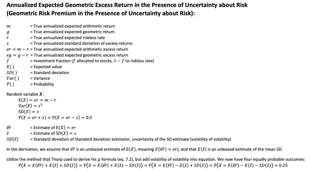
Annualized expected geometric excess return in the presence of uncertainty about risk

Ed Thorp derived a continuous variable continuous time version of the Kelly criterion in [1]. He first derived a formula for (continuously compounded) expected growth rate (equation 7.2). The starting point of his derivation was two equally likely returns, which deviated from the expected return by the amount of one standard deviation. We follow Thorp, but make our parameters random variables and include uncertainty of the risk (volatility of volatility) in the equation. Our starting point consists of four returns (two pairs) that are equally likely, and each pair deviates from the two returns Thorp used by the standard deviation of standard deviation.

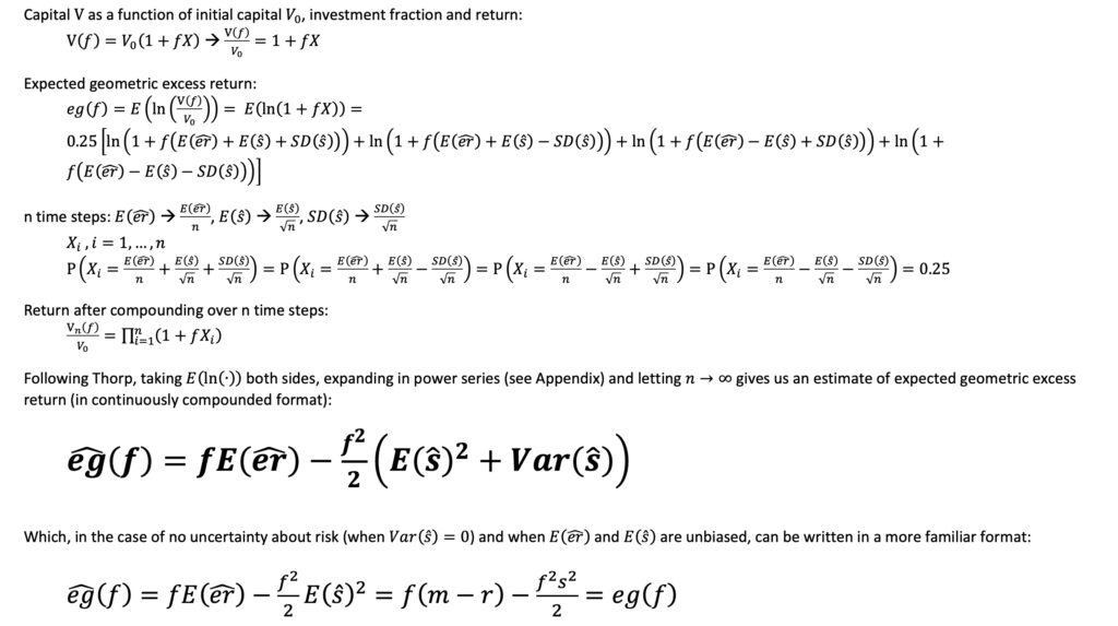
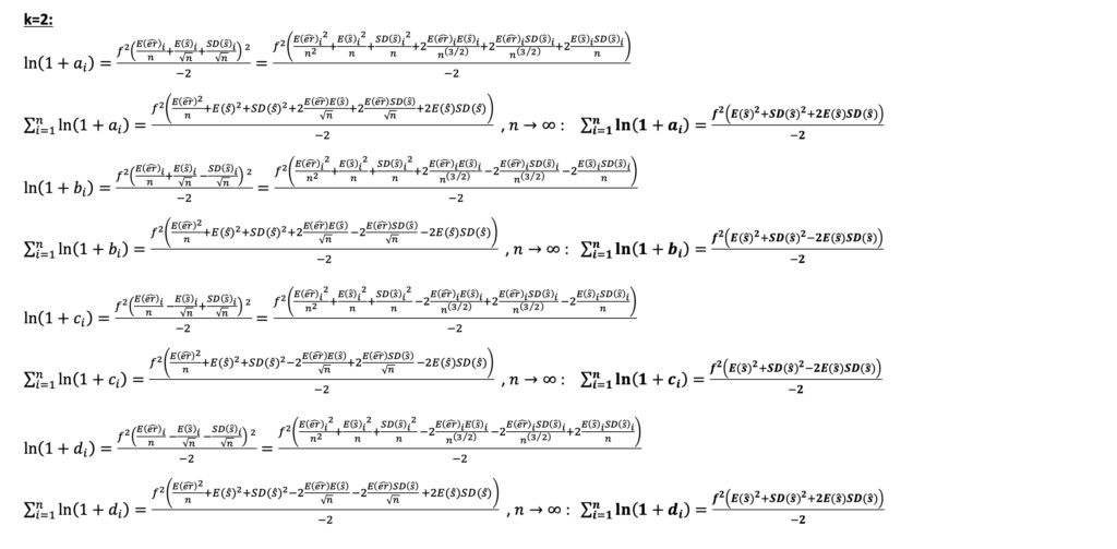
Thorp derived a formula for expected growth rate. We derive a formula for expected excess growth rate (growth rate in excess of riskless rate). This simplifies the derivation and we can incorporate the riskless rate into the equation post-derivation, if desired. The derivation itself follows Thorp’s approach and provides an estimate of expected geometric excess return when the input parameters are uncertain. Power series expansion is presented in the Appendix.

The key difference between the derived expected geometric excess return formula in the presence of uncertainty about risk and the version of the formula derived with known parameters, such as when calculating ex-post mean geometric excess return using historically realized parameters, is that the variance drag component of the formula now incorporates not only the square of expected volatility (consistent with the formula with known parameters) but also the variance of volatility (square of volatility of volatility). In essence, both risk (volatility) and the uncertainty related to risk (volatility of volatility) contribute to the reduction of expected geometric return.

Consequently, all else equal, the ex-ante estimate of expected growth rate (based on realized historical parameters) is lower than the ex-post (realized) mean growth rate.

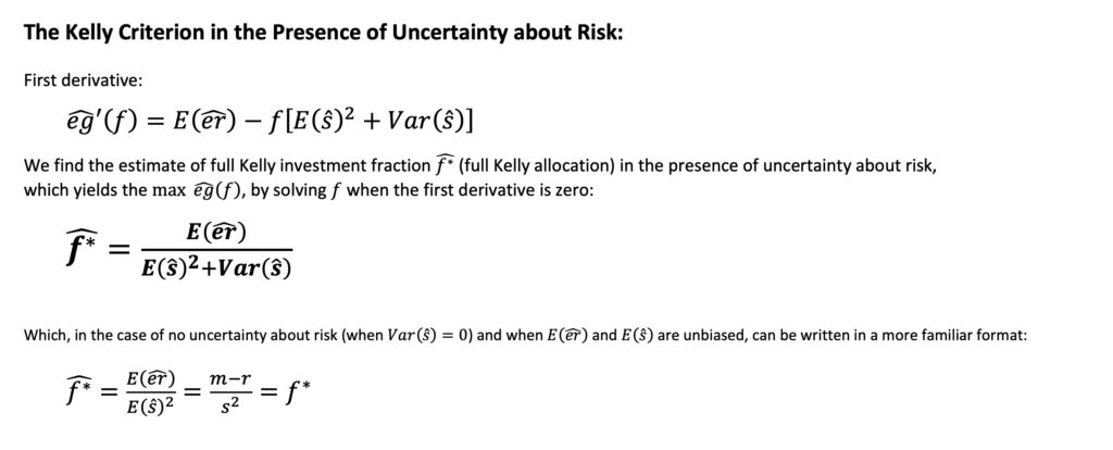
The Kelly criterion in the presence of uncertainty about risk

We next derive an estimate of the leverage multiplier that maximizes the expected growth rate, representing the Kelly criterion in the presence of uncertainty about risk. We observe that not only does the square of expected volatility (in line with the formula with known parameters) reduce the optimal Kelly leverage, but also the volatility of volatility (or more precisely, the variance of volatility) contributes to this reduction.

It follows that, all else equal, the ex-ante estimate of full Kelly leverage multiplier (based on realized historical parameters) is lower than the ex-post (realized) full Kelly leverage multiplier.

Volatility and Sharpe ratio in the presence of uncertainty about risk

More generally, we obtain an estimate of variance under uncertainty about risk as the sum of square of the expected volatility and the variance of volatility. We obtain an estimate of volatility under uncertainty about risk by taking the square root of estimate of variance under uncertainty about risk, which is an increasing function of variance of volatility.

We can then utilize the estimate of volatility under uncertainty about risk and derive an estimate of Sharpe ratio under uncertainty about risk, which is a decreasing function of variance of volatility.

Intuitively, in our imagination, we can string together all possible alternative return distributions (each with a different volatility) over time (with each return distribution broken down into a series of returns) and then calculate the volatility and Sharpe ratio over the entire time duration.

It follows that, all else equal, the ex-ante estimate of volatility (based on realized historical volatility) is higher and the ex-ante estimate of Sharpe ratio (based on realized historical parameters) is lower than the ex-post (realized) volatility and Sharpe ratio, respectively.

In my earlier article, The Kelly criterion, capital market parabola & the almighty Sharpe ratio, we derived fractional Kelly criterion formulas for known parameters. Formulas were expressed as functions of volatility and Sharpe ratio. We can use any of those formulas under uncertainty about risk by substituting volatility and Sharpe ratio with their uncertain estimates shown below.

Assuming individuals care about risk-adjusted returns or expected geometric growth rate, the observation that the Sharpe ratio, the expected growth rate and the leverage multiplier maximizing expected growth rate are all decreasing functions of uncertainty related to risk (volatility of volatility) implies that ambiguity aversion (preference for known risks over unknown risks) is perfectly rational.

Diversification premium in the presence of uncertainty about risk

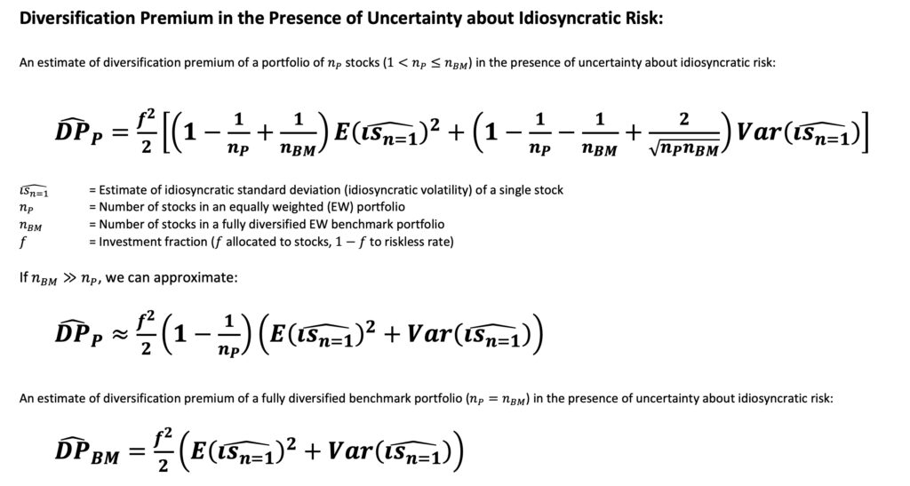
In my earlier article, Diversification is a negative price lunch, we introduced the concept of diversification premium using known parameters. Diversification premium represents the difference between expected geometric growth rate of a randomly selected portfolio and that of a randomly selected single stock. Our formula is applicable to equally weighted portfolios, essentially capturing the difference in variance drags.

Firm specific risk, idiosyncratic standard deviation, like any risk is subject to estimation uncertainty (volatility of idiosyncratic volatility). As shown below (formulas have been derived in section 3.3.9 of my thesis [2]), diversification premium is an increasing function of the uncertainty related to idiosyncratic risk. In essence, the more uncertainty there is about idiosyncratic risk, the more advantageous diversification becomes.

It follows that, all else equal, the ex-ante estimate of diversification premium (based on realized historical parameters) is higher than the ex-post (realized) diversification premium. 

Annualized expected geometric excess return in the presence of uncertainty about systematic and idiosyncratic risk

In my earlier article, Diversification is a negative price lunch, we explored the historical scenario where the cost of diversification was high, particularly before the advent of index funds and ETFs. This led to concentrated portfolios and low diversification premium, necessitating a higher ex-ante market-level return expectation to compensate for the lower expected growth rate resulting from limited diversification. In other words, we argued that frictions preventing full diversification should have necessitated a higher return requirement. This, in turn, should have resulted in a higher overall market return than if diversification had been easier.

Under uncertainty about both systematic and idiosyncratic risk, we have four components all contributing to higher variance drag and lower risk adjusted return: 1) square of expected systematic volatility, 2) variance of systematic volatility, 3) square of expected idiosyncratic volatility and 4) variance of idiosyncratic volatility. These aspects are captured in the estimate of geometric risk premium and Sharpe ratio formulas under uncertainty about systematic and idiosyncratic risk below.

Assuming investors care about risk-adjusted returns and/or expected growth rate, it’s important to note that not only risk but also uncertainty related to risk warrants a premium. This observation can provide a partial explanation for the equity premium puzzle.

Furthermore, under uncertainty about idiosyncratic risk, there are two reasons why under-diversified investors of the past should have had a higher ex-ante return requirement compared to investors today who have access to virtually free diversification: 1) expected idiosyncratic volatility and 2) uncertainty (variance) related to the idiosyncratic volatility estimate. The effect of uncertainty related to idiosyncratic risk helps us explain the equity premium puzzle in history when cheap diversification was not possible.

Empirical demonstrations

U.S. stock exchanges, based on Kenneth French’s daily stock market data [3], transitioned from six days a week of trading to five days a week at the beginning of June 1952. We utilize daily excess return data starting from June 1952, benefiting from the relatively constant 252 (an average of 251.7) trading days per year since that time. 252 translates to about 21 trading days per month. We use the annualized volatility of a 21-day period as a proxy for monthly volatility. 

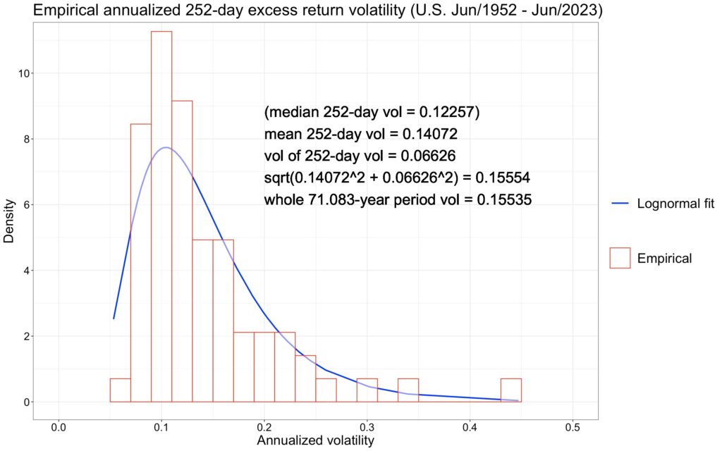
The figure below illustrates the distribution of volatility for all non-overlapping 21-day periods. Our formula for estimating volatility in the presence of uncertainty about risk works well empirically. It’s noteworthy that the distribution shape is not symmetric but positively skewed. While the log-normal distribution may not be a perfect fit, it serves as a relatively good model for volatility.

The positive skewness implies that the median (typical) monthly volatility is considerably lower than the mean monthly volatility and even more so compared to long-term (71.25-year) volatility, which is increased by volatility of volatility. Any randomly picked realized short-term volatility is likely to underestimate the long-term volatility. Additionally, a relatively large portion of the long-term volatility is attributed to rare high-volatility months in the right tail.

The next figure illustrates the distribution of volatility for all non-overlapping 252-day (yearly) periods. Once again, our formula for estimating volatility in the presence of uncertainty about risk proves effective empirically.

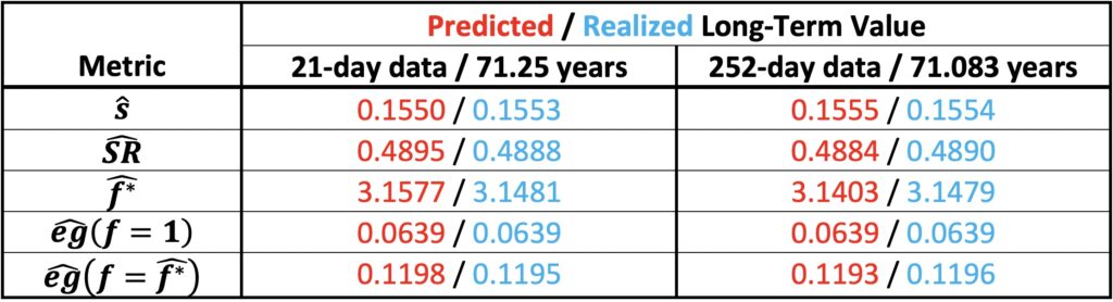
The volatility estimate in the presence of uncertainty about risk serves as the foundation for our formulas, which estimate various metrics. We can empirically test our formulas as uncertainty resolves over the long term in our empirical data, eventually reaching a sample size of one and resulting in a single realized long-term value. The table below demonstrates that our formulas accurately predict empirically realized long-term metrics from short-term data when assuming an unbiased mean excess return estimate (utilizing the empirically realized value of 0.0760).

We can conduct a thought experiment where the stock market only has one year of history. There is a 50%/50% chance that the volatility is lower/higher than the median yearly volatility. The same applies to mean excess returns and the Sharpe ratio. If we assume that both excess return volatility and mean excess return were at their median values (0.1226 and 0.0886, respectively), the investor equipped with one year of market data would calculate his naïve forward-looking estimates based on realized parameters:

• Sharpe ratio: 0.0886/0.1226 = 0.7227
• Optimal full Kelly leverage multiplier: 0.7227/0.1226 = 5.895
• Expected unleveraged excess growth rate: 0.0886 – (0.1226^2)/2 = 0.0811
• Max expected excess growth rate (at full Kelly leverage): (0.7227^2)/2 = 0.2611

Alternatively, we can select the historical median Sharpe ratio of 0.6796 (with volatility = 0.1456 and mean excess return = 0.0990). This would result in forward-looking estimates based on realized parameters:

• Sharpe ratio: 0.6796
• Optimal full Kelly leverage multiplier: 0.6796/0.1456 = 4.668
• Expected unleveraged excess growth rate: 0.0990 – (0.1456^2)/2 = 0.0884
• Max expected excess growth rate (at full Kelly leverage): (0.6796^2)/2 = 0.2309

While the same metrics, empirically after over 71 years of data, result in:

• Sharpe ratio: 0.0760/0.1554 = 0.4891
• Optimal full Kelly leverage multiplier: 0.4891/0.1554 = 3.147
• Expected unleveraged excess growth rate: 0.0760 – (0.1554^2)/2 = 0.0639
• Max expected excess growth rate (at full Kelly leverage): (0.4891^2)/2 = 0.1196

We can observe that, no matter if we are using median volatility and median mean excess return metrics or the median Sharpe ratio from short-term (yearly) data, all the derived metrics grossly exaggerate the return and leveraging opportunities, as well as the risk-adjusted return, when compared against realized long-term metrics.

There are essentially two reasons for the overestimation: 1) the uncertainty of forward-looking risk (variance of volatility) needs to be taken into account, as we have discussed, and 2) the positively skewed distribution of volatility, indicating that most observations are below the mean. The second reason implies that our estimate of expected volatility is likely a biased underestimate when using historical realized volatility as our guide. In our empirical data, the probability that a randomly selected yearly volatility is lower than the mean yearly volatility is 63.4%, while the probability that yearly volatility is lower than the full 71-year period volatility is 69.0%. The positively skewed shape of the volatility distribution persists across any time horizon, given that the downside of volatility is limited to zero while the upside can expand without limitations.

Additionally, both monthly and yearly empirical mean excess return distributions display negative skewness (with most observations above the mean). This suggests that our estimate of mean excess return is likely a biased overestimate when extrapolating historical realized short-term mean excess return into the future.

Uncertainty can arise, for example, from a small sample size or from population parameters being time-variant (data not being stationary). One might argue that our thought experiment cannot be generalized to longer horizons, as one year of data can clearly be considered a small sample, and we should assume that sample size-related uncertainty is greatly suppressed as we add a lot more data (e.g., utilizing 10-year or 100-year periods instead of yearly periods). However, we could similarly argue that population uncertainty increases as the time horizon lengthens. It is not clear at all that uncertainty should decrease as we consider longer and longer time horizons. Our point is that any uncertainty, regardless of its origin, is detrimental to geometric return metrics.

Simulations

The figure below illustrates how expected excess growth rate and optimal full Kelly leverage under uncertainty about risk behave as a function of leverage. We assume that the cost of leverage is equal to the riskless rate and that the portfolio is rebalanced to target leverage at infinite frequency. In this simulation, we randomly draw 250,000 10-year returns from a log-normal distribution and calculate the annualized return (log return). We run the simulation independently for each leverage multiplier with a step size of 0.025.

Mean excess return is set to 0.08, and volatility (or mean volatility when volatility of volatility is present) is set to 0.20. With these parameters, the unleveraged expected excess growth rate is calculated as 0.08 – (0.2^2)/2 = 0.06. The full Kelly leverage is determined as 0.08/(0.2^2) = 2, and the maximum expected excess growth rate (at full Kelly leverage) is ((0.08/0.2)^2)/2 = 0.08. In the figure, the black curve represents the scenario without uncertainty related to risk (volatility of volatility is zero) and we can see the values calculated above realized for this curve.

However, the red and blue curves introduce uncertainty about risk. The volatility of volatility is simulated by randomly drawing the volatility for each 10-year log-normal distribution, where the 10-year return is drawn. The drawn volatilities are from a log-normal distribution with a mean of 0.20 and a standard deviation of 0.10 for the red curve or 0.20 for the blue curve. As depicted in the figure, the uncertainty in the volatility estimate (volatility of volatility) leads to a decrease in the expected excess growth rate and full Kelly leverage multiplier. The simulated curves align closely with the theoretical predictions derived from our equations.

Furthermore, our simulation involves drawing the mean excess return for each 10-year period from a normal distribution with a mean of 0.08 and a standard deviation of 0.20. This is done to simulate the non-stationarity of the mean excess return, although it doesn’t impact the simulation result. We tested and confirmed that the result remains the same both with and without a constant mean excess return, as the uncertainty related to the (unbiased) mean excess return averages out.

Additionally, we conducted tests introducing uncertainty by varying both the mean volatility and the volatility of volatility in the simulation. The outcome of these supplementary tests indicated that regardless of the source of uncertainty related to risk, it all manifests in the volatility of volatility metric. In essence, the variance of volatility comprises (the sum of) all variances associated with volatility, whether arising from the non-stationarity of mean volatility, volatility of volatility, volatility of volatility of volatility, and so forth. Introducing all these uncertainties does make the simulation time requirement very high as it takes a very long time for the result to converge under multiple time varying uncertainties.

The simulation is intended to illustrate the negative effects of uncertainty related to risk, rather than to establish specific levels of uncertainty (0.10 and 0.20, chosen for visible impact) associated with the 10-year horizon risk.

Our simulation highlights why investors should be wary of volatility of volatility. It underscores the potential advantages of diversifying not only across assets but also across different asset classes and strategies to mitigate not only risk (volatility) but also uncertainty related to risk (volatility of volatility).

Our equations establish a theoretical foundation, and simulations indicate potential benefits from tail hedging. While tail hedging comes with a cost, it has the potential to limit (and consequently reduce) both expected risk and uncertainty related to risk, thereby enhancing the expected growth rate and creating opportunities for leveraging.

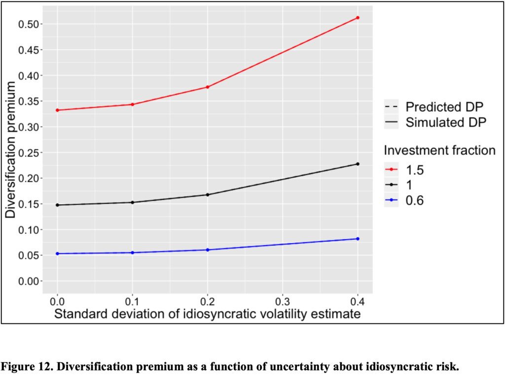
Lastly, we explore the impact of idiosyncratic volatility on the diversification premium of a fully diversified equally weighted portfolio. The simulation, detailed in section 4.2.1.3 of my thesis [2], is illustrated in the figure below.

Our simulation uses the idiosyncratic standard deviation of a single stock, which is 0.5434 and is derived from CRSP data for the U.S. stock market covering the period from Jan-1973 to Jun-2018. This dataset encompasses all common stocks, the majority of which are micro caps, with an average of 5472 stocks per month. To conduct our simulation, we generate and aggregate 20 sets of data, each spanning 500 years (totalling 10,000 years) on a monthly basis, with each dataset comprising monthly returns from 5472 firms.

The annualized unleveraged diversification premium (in the absence of uncertainty related to idiosyncratic risk) for a fully diversified equally weighted benchmark portfolio is calculated as (0.5434^2)/2, resulting in 0.1476. The figure below illustrates how the diversification premium increases with uncertainty related to idiosyncratic risk. Simulated results align perfectly with theoretical values predicted by our equations.

Conclusions & implications

We know historically realized risk as a fact, but estimates of future risk always involve uncertainty. This uncertainty related to risk reduces estimates of the unleveraged expected growth rate, maximum achievable expected growth rate, optimal full Kelly leverage, and, more generally, increases the estimate of volatility while decreasing the estimate of Sharpe ratio.

Uncertainty related to firm-specific risk, however, increases the estimated future diversification benefit, manifesting as the potential for a larger reduction in idiosyncratic volatility through diversification and a higher diversification premium.

Our results suggest that measures with the potential to reduce not only risk but also uncertainty related to risk, such as diversification across asset classes and strategies, as well as tail risk hedging, may enhance risk-adjusted returns, expected growth rates, and leveraging opportunities for a portfolio.

The volatility estimate is derived as the square root of the sum of the squared expected volatility and the variance of volatility, representing the uncertainty related to risk. This uncertainty, importantly, contributes to an increase in the volatility estimate. Moreover, owing to the positively skewed shape of the volatility distribution, the expected volatility estimate based on historical realized volatility is likely to be biased, tending to underestimate the expected value of the future volatility. This, in turn, further downplays the overall volatility estimate.

All else being equal, this implies that the estimated forward-looking expected growth rate (ex-ante geometric risk premium) and optimal leverage are lower than the historically realized mean growth rate (ex-post geometric risk premium) and optimal leverage. However, the estimated diversification benefit exceeds the historically realized diversification benefit.

Furthermore, in the past, cheap and easy diversification was not available to investors. Consequently, investors had to bear both systematic and firm-specific risk. The uncertainty related to both of these risks should have increased the ex-ante expected growth rate requirement. Both uncertainties about systematic and idiosyncratic risk contribute to explaining the (geometric) equity premium puzzle.

Assuming investors care about risk-adjusted returns or expected geometric growth rates, the observation that uncertainty about risk is detrimental to estimates of Sharpe ratio and geometric metrics, such as expected growth rate and optimal full Kelly leverage, implies that ambiguity aversion is not an irrational behavioural bias. Instead, it appears to be perfectly rational behaviour.

References

[1] Thorp, E. O. (2006). The Kelly criterion in blackjack, sports betting and the stock market

• For instantaneous geometric expected return, see derivation of eq. 7.2

[2] Kurtti, M. T. (2020). How many stocks make a diversified portfolio in a continuous-time world?

• 3.3.9    Derivation of diversification premium under uncertainty about risk
• 4.2.1.3  Simulation of diversification premium under uncertainty about risk

 [3] Kenneth French. Fama/French 3 Factors [Daily]

Appendix

Article by Markku Kurtti